---
title: "Multi-Fidelity Statistical Estimation on an Aerospace Structure"
subtitle: "PyApprox Tutorial Library"
description: "An end-to-end worked example: estimating statistics of a wing-spar reliability QoI with group ACV on a deliberately partially ordered ensemble (nonlinear-elasticity reference, linear-elasticity reductions, and a polynomial-chaos surrogate) that shares one parameterization, with measured costs and a pilot-estimated covariance."
tutorial_type: usage
topic: multi_fidelity
difficulty: intermediate
estimated_time: 20
render_time: 300
prerequisites:
- group_acv_concept
- group_acv_mixed_concept
- multifidelity_estimation_cookbook
- kle_introduction
tags:
- multi-fidelity
- group-acv
- aerospace
- case-study
- finite-element
format:
html:
code-fold: false
code-tools: true
toc: true
execute:
echo: true
warning: false
jupyter: python3
---
::: {.callout-tip collapse="true"}
## Download Notebook
[Download as Jupyter Notebook](notebooks/multifidelity_aerospace_beam.ipynb)
:::
## Learning Objectives
After completing this tutorial, you will be able to:
- Assemble a deliberately **partially ordered** multi-fidelity ensemble — mixing
reduced physics, a coarsened mesh, and a surrogate — that shares one input
parameterization so the models are correlated
- Measure per-model **costs** and estimate the cross-model **covariance** from a
pilot study on a real (non-analytic) ensemble
- Predict and compare the variance of MC, MLMC, and **group ACV**
estimators at fixed budget, without needing a closed-form truth
- Add a **surrogate with a known mean** and quantify the extra variance reduction
(mixed known statistics)
- Estimate **two quantities of interest jointly** (deflection and stress) with
multi-output group ACV
## Prerequisites
This tutorial applies [Group ACV Concept](group_acv_concept.qmd),
[Group ACV Mixed Concept](group_acv_mixed_concept.qmd), and the
[Multi-Fidelity Estimation Cookbook](multifidelity_estimation_cookbook.qmd) to a
realistic physics ensemble. It uses a Karhunen–Loève random field; see
[KLE Introduction](kle_introduction.qmd).
## Motivation: Reliability of a Wing Component
Certifying an aircraft requires quantifying the **structural reliability** of its
load-carrying members under uncertain loads and material properties. The
high-fidelity models are coupled aero-structural simulations costing hours per
run — far too expensive to sample the thousands of times a Monte Carlo
reliability estimate needs.
Multi-fidelity statistical estimation combines a few expensive high-fidelity
evaluations with many cheap low-fidelity ones to estimate the high-fidelity
statistic **without bias** at a fraction of the cost. This tutorial uses a cheap
stand-in that preserves the multi-fidelity *structure* of the real problem: a
composite **wing-spar panel** with lightening holes, clamped at the root and
loaded along its top edge. We estimate two reliability-relevant quantities of
interest:
- **Tip deflection** $\delta$ — a stiffness/serviceability measure.
- **Peak (or area-integrated) von Mises stress** $\sigma$ — a strength-margin
measure; the holes make this respond to the random field, not just the load.
## A Problem, Not a Benchmark
The analytic ensembles used elsewhere in the library (polynomial, tunable) are
**benchmarks**: their means and covariance are known in closed form, so estimator
error can be plotted against a true value. This finite-element ensemble has **no
closed-form truth**, so it is a **problem**, not a benchmark.
This matters less than it might seem. The headline multi-fidelity result —
estimator variance versus cost — depends only on the model **covariance** and the
**sample allocation**, both of which we have: the covariance is estimated from a
pilot, and the variance of each estimator is then a known function of that
covariance. We do not need a truth value to produce the variance-vs-cost curve.
No large-sample Monte Carlo reference is needed for the headline result.
::: {.callout-note}
A closed-form-truth variant is possible in low input dimension via tensor-product
quadrature on the model functions, which would let estimators be shown converging
to a known value. That is deferred; this tutorial stays with the realistic
problem and predicts estimator variance from the pilot covariance.
:::
## The Ensemble: Partially Ordered by Design
| Index | Model | Reduction | Nominal cost |
|:-:|---|---|:-:|
| 0 | 2D **Neo-Hookean** (nonlinear), fine mesh | HF reference | $1$ |
| 1 | 2D **linear** elasticity, same fine mesh | physics | $\sim 0.3$ |
| 2 | 2D **linear** elasticity, coarse mesh | physics + mesh | $\sim 0.02$ |
| 3 | **PCE surrogate** of model 0 (known mean) | data-fit | $\sim 10^{-5}$ |
The ordering is intentionally incomplete. Models 2 and 1 are a clean refinement
pair (same physics, finer mesh). Model 1 versus model 0 is *load-dependent*: at
low load the linear and nonlinear responses nearly coincide ($\rho \to 1$); at
high load geometric stiffening makes them diverge. Model 3, a data-fit surrogate,
is not comparable to the mesh models at all — its accuracy depends on training,
not discretization — and it enters through its **analytic mean** rather than by
sampling. This is precisely the partially ordered setting that group ACV handles
and a strict hierarchy (MLMC) does not.
## Parameterizing the Uncertainty
Every model consumes the same input
$\boldsymbol{\theta} = (\xi_1, \ldots, \xi_d, q_0)$:
- $\xi \in \mathbb{R}^d$ are standard-normal coefficients of a **spanwise
log-Young's-modulus field** $\log E(x)$, a $d$-term KLE defined once on the
reference span and broadcast through the section, so 2D and surrogate all see
the same realization. We take $d = 5$ (small, which also keeps a future
quadrature-truth variant tractable).
- $q_0$ is a **random load magnitude** scaling the top-edge traction.
## Building the Ensemble
The `CantileverBeamEnsembleProblem` assembles the four-model ensemble.
Each FEM model uses a shared KLE for the Young's modulus field on its own mesh
and accepts a random wind speed as input. The traction load is the dynamic
pressure $q_0 = v^2$, so the input-to-output map is nonlinear for all models.
Models are wrapped with `make_parallel` for multi-core evaluation and `timed`
for cost measurement.
```{python}
import numpy as np
from pyapprox.util.backends.numpy import NumpyBkd
from pyapprox_benchmarks.statest import CantileverBeamEnsembleProblem

bkd = NumpyBkd()
np.random.seed(42)

NUM_KLE_TERMS = 5

ensemble = CantileverBeamEnsembleProblem(
    bkd,
    num_kle_terms=NUM_KLE_TERMS,
    sigma=1.0,
    fine_mesh_h=1,
    coarse_mesh_h=2,
    wind_s=0.5,
    wind_scale=2.5,
    n_jobs=-1,
)

prior = ensemble.prior()
models = ensemble.models()
model_names = ensemble.model_names()
nmodels_fem = len(models)  # 3 FEM models initially
print(f"{nmodels_fem} FEM models built, nvars = {NUM_KLE_TERMS + 1}")
```
## Training the PCE Surrogate
We train a polynomial chaos expansion (PCE) surrogate of the high-fidelity
model (f0) on a **separate** sample set — not the pilot — to avoid artificially
inflating the surrogate-to-HF correlation in the pilot covariance estimate.
The PCE's analytic mean enters via `known_quantities`.
```{python}
NTRAIN = 14
train_samples = prior.rvs(NTRAIN)
train_values_f0 = models[0](train_samples)

pce = ensemble.fit_pce_surrogate(
    train_samples, train_values_f0, max_level=1, cv_levels=[1],
)

pce_mean = ensemble.pce_mean()
print(f"PCE analytic mean: deflection={bkd.to_numpy(pce_mean)[0]:.4f}, "
      f"stress={bkd.to_numpy(pce_mean)[1]:.1f}")
print(f"Ensemble now has {ensemble.nmodels()} models")
```
## The Pilot Study
The pilot evaluates **every model at the same inputs** to estimate the
cross-model covariance. Because models are wrapped with `timed`, we also
extract the measured per-sample costs after evaluation.
```{python}
from pyapprox.statest.statistics import MultiOutputMean

NPILOT = 50
pilot_samples = prior.rvs(NPILOT)
pilot_values = [m(pilot_samples) for m in ensemble.models()]

nqoi = 2
stat = MultiOutputMean(nqoi, bkd)
cov_pilot, = stat.compute_pilot_quantities(pilot_values)
stat.set_pilot_quantities(cov_pilot)

nmodels = ensemble.nmodels()

# Extract measured costs
costs = ensemble.extract_costs()
costs_np = bkd.to_numpy(costs)
print("Measured costs (normalized to f0 = 1):")
for name, c in zip(ensemble.model_names(), costs_np):
    print(f"  {name}: {c:.6f}")
```
```{python}
# Inspect pilot correlations with HF model
cov_np = bkd.to_numpy(cov_pilot)
qoi_names = ["Tip deflection", "Integrated VM stress"]
print("\nPilot correlations with f0:")
for qi, qname in enumerate(qoi_names):
    print(f"  {qname}:")
    for a in range(1, nmodels):
        ii, jj = qi, a * nqoi + qi
        rho = cov_np[ii, jj] / np.sqrt(cov_np[ii, ii] * cov_np[jj, jj])
        print(f"    ρ(f0, f{a}) = {rho:.4f}")

pilot_values_np = [bkd.to_numpy(pv) for pv in pilot_values]
```
## Visualizing the Ensemble
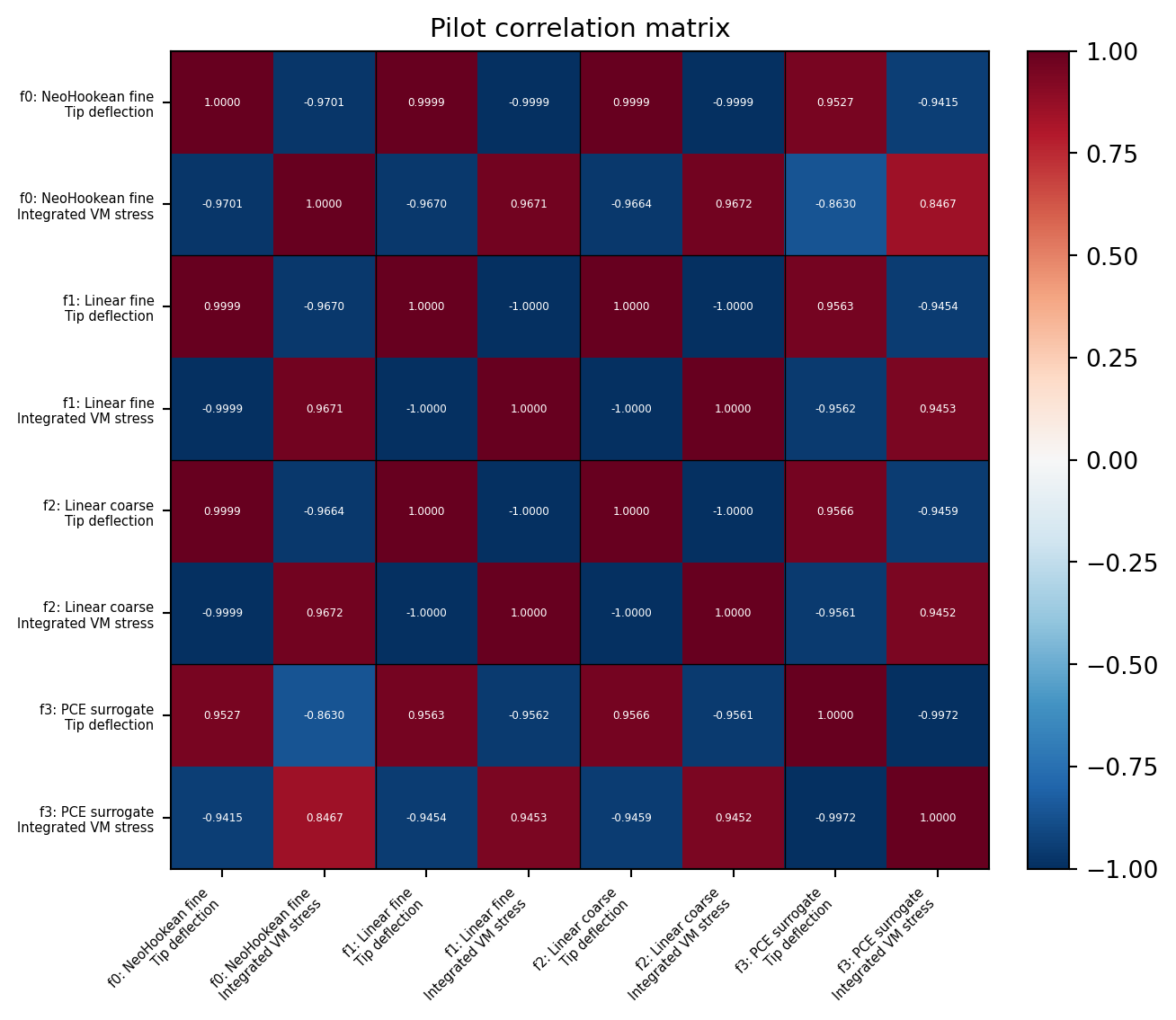
The pilot data reveals the inter-model structure that group ACV exploits.
The correlation heatmap (@fig-correlation-heatmap) shows the full
`(nmodels × nqoi)` pilot covariance: linear-elasticity models correlate
strongly with the HF for deflection but less for stress, and the PCE
surrogate (trained on separate data) inherits the HF's variance structure
but not perfectly.
```{python}
#| echo: false
#| fig-cap: "Pilot correlation matrix over all (model, QoI) pairs. Block boundaries separate models; within each block the two QoIs (deflection, stress) may be cross-correlated. The partial ordering is visible: f1 and f2 correlate more strongly for deflection than for stress, while the PCE surrogate (f3) has near-perfect correlation for deflection but lower for stress."
#| label: fig-correlation-heatmap
import matplotlib.pyplot as plt
from pyapprox_tutorials.figures._aerospace_beam import (
plot_pilot_correlation_heatmap,
)
fig, ax = plt.subplots(1, 1, figsize=(7, 6))
plot_pilot_correlation_heatmap(
ax, cov_np, nmodels, nqoi, ensemble.model_names(), qoi_names,
)
ax.set_title("Pilot correlation matrix", fontsize=11)
fig.tight_layout()
plt.show()
```
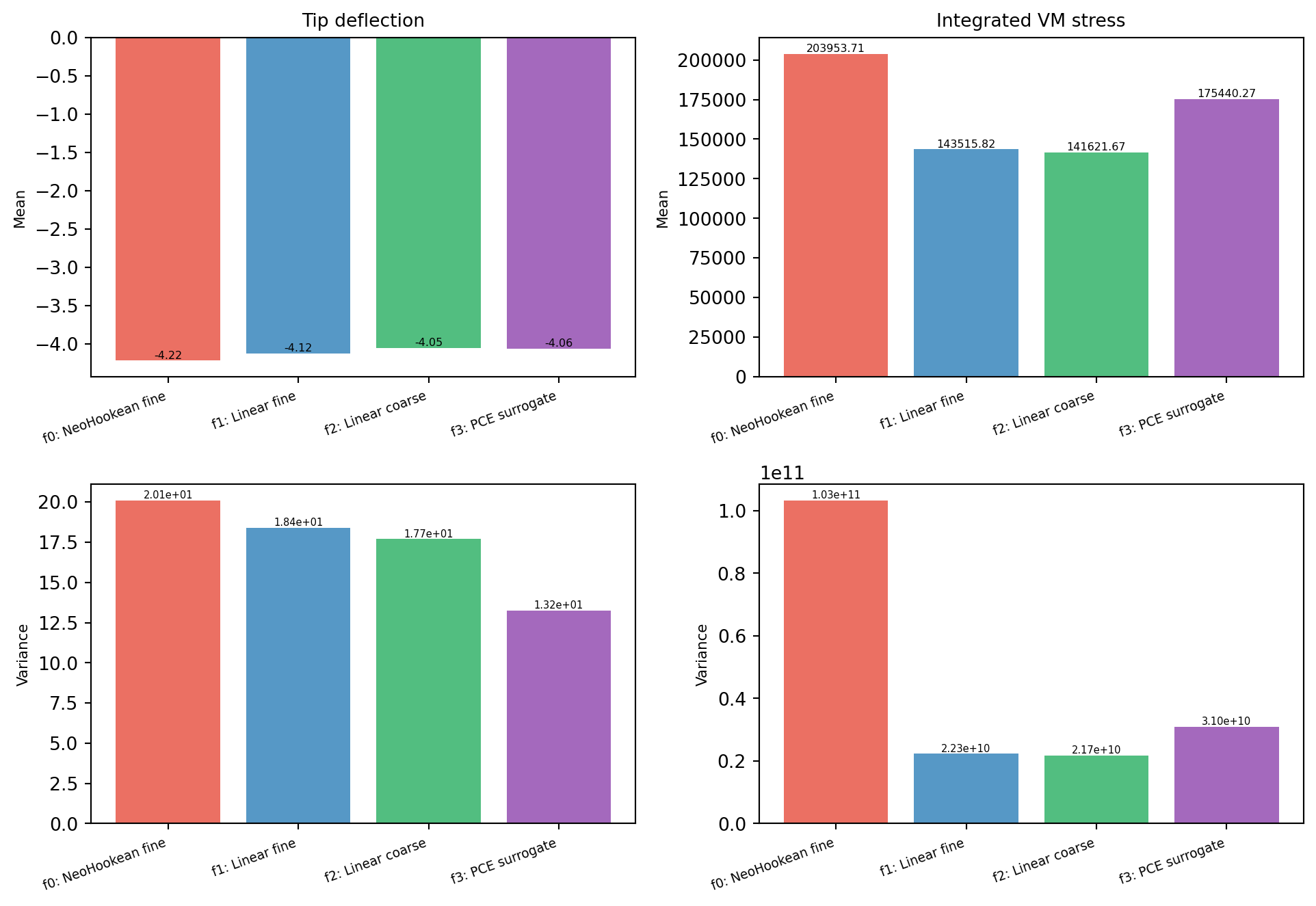
The per-model means and standard deviations (@fig-means-variances) quantify
**bias**: the low-fidelity models approximate the HF response but do not match
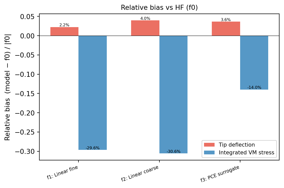
it exactly. @fig-bias shows the bias relative to the HF explicitly. The CV
framework corrects for this bias, but the further a model's mean is from the HF,
the larger the control-variate correction.
```{python}
#| echo: false
#| fig-cap: "Per-model pilot means (top) and variances (bottom) for each QoI. The bias of each low-fidelity model relative to f0 is visible in the means; the variances show the output spread that drives the covariance structure."
#| label: fig-means-variances
from pyapprox_tutorials.figures._aerospace_beam import (
plot_pilot_means_and_variances,
)
fig, axes = plt.subplots(2, 2, figsize=(10, 7))
plot_pilot_means_and_variances(
axes, pilot_values_np, ensemble.model_names(), qoi_names,
)
fig.tight_layout()
plt.show()
```
```{python}
#| echo: false
#| fig-cap: "Relative bias (model mean − f0 mean) / |f0 mean| for each low-fidelity model, grouped by QoI. Normalizing by the HF mean puts both QoIs on the same scale and shows that biases are a few percent — small enough for effective control-variate correction."
#| label: fig-bias
from pyapprox_tutorials.figures._aerospace_beam import plot_bias_vs_hf
fig, ax = plt.subplots(1, 1, figsize=(6, 4))
plot_bias_vs_hf(ax, pilot_values_np, ensemble.model_names(), qoi_names)
ax.set_title("Relative bias vs HF (f0)", fontsize=10)
fig.tight_layout()
plt.show()
```
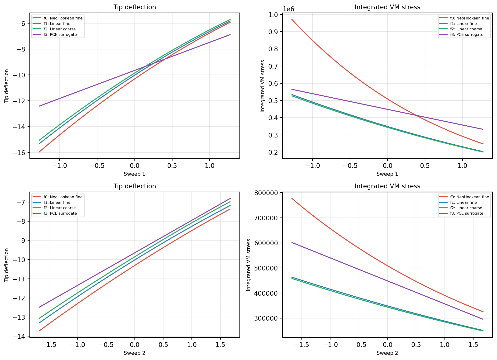
A 1D parameter sweep along random directions through the full input space
(@fig-1d-sweep) reveals where models track the HF closely and where they
diverge. Each sweep varies all six inputs simultaneously along a random
direction, correctly handling the mixed normal/lognormal parameterization
via the isoprobabilistic transform.
```{python}
#| echo: false
#| fig-cap: "Response of all four models along two random directions through the 6D input space. Each sweep varies all inputs simultaneously; the x-axis is the distance along the sweep direction. The linear models closely track the nonlinear HF for deflection, but stress diverges along directions that excite geometric nonlinearity. The PCE surrogate smoothly approximates f0 over the training range."
#| label: fig-1d-sweep
from pyapprox.interface.functions.sweeps import MarginalParameterSweeper
from pyapprox_tutorials.figures._aerospace_beam import plot_1d_sweep
marginals = list(ensemble.prior().marginals())
sweeper = MarginalParameterSweeper(
marginals, sweep_radius=2.5, nsamples_per_sweep=40, bkd=bkd,
)
NSWEEPS = 2
np.random.seed(123)
sweep_samples = sweeper.rvs(nsweeps=NSWEEPS)
canonical = bkd.to_numpy(sweeper.canonical_active_samples())
NSWEEP = sweeper.nsamples_per_sweep()
sweep_vals = [[] for _ in range(NSWEEPS)]
for m in ensemble.models():
all_vals = bkd.to_numpy(m(sweep_samples))
for s in range(NSWEEPS):
sweep_vals[s].append(all_vals[:, s * NSWEEP:(s + 1) * NSWEEP])
fig, axes = plt.subplots(2, 2, figsize=(11, 8))
for s in range(NSWEEPS):
plot_1d_sweep(
axes[s], canonical[s], sweep_vals[s],
ensemble.model_names(), qoi_names,
)
axes[s][0].set_xlabel(f"Sweep {s + 1}", fontsize=8)
axes[s][1].set_xlabel(f"Sweep {s + 1}", fontsize=8)
fig.tight_layout()
plt.show()
```
::: {.callout-note}
Re-run the pilot at several `NPILOT` and watch the predicted group ACV variance
stabilize: on a real ensemble the covariance is estimated, so the allocation and
the predicted variances are themselves uncertain (see
[Pilot Studies](pilot_studies_concept.qmd)).
:::
## Building and Comparing Estimators
With costs and covariance in hand, we compare MC against group ACV (full
subsets) for **two statistics** — the mean and the variance — on each QoI
independently. For the mean we also compare against joint 2-QoI estimation,
which exploits cross-QoI covariance for free variance reduction. Each
configuration is tested with and without the PCE's known statistics.
```{python}
from pyapprox.statest.groupacv import (
    GroupACVEstimatorIS,
    FittedGroupACVEstimator,
    get_model_subsets,
    MeanGuidedSubsetFitter,
)
from pyapprox.statest.groupacv.allocation import GroupACVAllocationOptimizer
from pyapprox.statest.groupacv.variable_space import AllocationProblemConfig
from pyapprox.statest.statistics import MultiOutputVariance
from pyapprox.optimization.minimize.scipy.slsqp import ScipySLSQPOptimizer

log_ineq = AllocationProblemConfig(
    variable_scaling="log", budget_constraint_form="inequality",
)
full_subsets = get_model_subsets(nmodels, bkd)
known_quantities = ensemble.known_quantities()
pce_var_np = bkd.to_numpy(pce.variance())

target_costs = np.array([50.0, 200.0, 1000.0])
optimizer = ScipySLSQPOptimizer(maxiter=1000, ftol=1e-6)

def _optimize_mean(stat_obj, kq, tc):
    """Optimize GACV for a mean stat and return predicted variance."""
    est = GroupACVEstimatorIS(
        stat_obj, costs, model_subsets=full_subsets, known_quantities=kq,
    )
    alloc = GroupACVAllocationOptimizer(
        est, optimizer=optimizer, problem_config=log_ineq,
    )
    res = alloc.optimize(tc, min_nhf_samples=2)
    if res.success:
        fitted = FittedGroupACVEstimator(est, res)
        return float(bkd.to_numpy(fitted.covariance()[0, 0]))
    return None

def _optimize_variance(stat_obj, kq, tc):
    """Mean-guided GACV for a variance stat, optionally with known quantities."""
    fitter = MeanGuidedSubsetFitter(
        stat_obj, costs, GroupACVEstimatorIS,
        candidate_subsets=full_subsets,
        optimizer=optimizer,
        problem_config=log_ineq,
        known_quantities=kq,
    )
    try:
        guided = fitter.fit(tc, min_nhf_samples=2)
    except RuntimeError:
        return None
    return float(bkd.to_numpy(
        guided.best_estimator.covariance()[0, 0]
    ))

# ---- Per-QoI mean and variance stats (nqoi=1 each) ----
all_results = {}
kq_mean_full = known_quantities[(3, "mean")]

for qi, qname in enumerate(qoi_names):
    pv_qi = [v[qi:qi+1, :] for v in pilot_values]

    # Mean stat
    stat_m = MultiOutputMean(1, bkd)
    cov_m, = stat_m.compute_pilot_quantities(pv_qi)
    stat_m.set_pilot_quantities(cov_m)
    kq_m = {(3, "mean"): bkd.array([bkd.to_numpy(kq_mean_full)[qi]])}

    # Variance stat
    stat_v = MultiOutputVariance(1, bkd)
    cov_v, W_v = stat_v.compute_pilot_quantities(pv_qi)
    stat_v.set_pilot_quantities(cov_v, W_v)
    kq_v = {
        (3, "mean"): bkd.array([bkd.to_numpy(kq_mean_full)[qi]]),
        (3, "variance"): bkd.array([pce_var_np[qi]]),
    }

    # Mean estimation (direct optimizer)
    mc_vals, gacv_vals, gacv_kn_vals = [], [], []
    for tc in target_costs:
        nhf = tc / costs_np[0]
        mc = float(bkd.to_numpy(
            stat_m.high_fidelity_estimator_covariance(
                bkd.array([nhf])
            )[0, 0]
        ))
        mc_vals.append(mc)
        gacv_vals.append(_optimize_mean(stat_m, None, tc) or mc)
        gacv_kn_vals.append(_optimize_mean(stat_m, kq_m, tc) or mc)
    all_results[("mean", qi)] = {
        "MC": mc_vals, "GACV": gacv_vals, "GACV + known": gacv_kn_vals,
    }

    # Variance estimation (mean-guided fitter)
    mc_vals, gacv_vals, gacv_kn_vals = [], [], []
    for tc in target_costs:
        nhf = tc / costs_np[0]
        mc = float(bkd.to_numpy(
            stat_v.high_fidelity_estimator_covariance(
                bkd.array([nhf])
            )[0, 0]
        ))
        mc_vals.append(mc)
        gacv_vals.append(_optimize_variance(stat_v, None, tc) or mc)
        gacv_kn_vals.append(_optimize_variance(stat_v, kq_v, tc) or mc)
    all_results[("variance", qi)] = {
        "MC": mc_vals, "GACV": gacv_vals, "GACV + known": gacv_kn_vals,
    }

# ---- Joint 2-QoI mean estimation ----
stat_joint = MultiOutputMean(nqoi, bkd)
stat_joint.set_pilot_quantities(cov_pilot)

for qi in range(nqoi):
    joint_vals = []
    for tc in target_costs:
        est = GroupACVEstimatorIS(
            stat_joint, costs, model_subsets=full_subsets,
            known_quantities=known_quantities,
        )
        alloc = GroupACVAllocationOptimizer(
            est, optimizer=optimizer, problem_config=log_ineq,
        )
        res = alloc.optimize(tc, min_nhf_samples=2)
        if res.success:
            fitted = FittedGroupACVEstimator(est, res)
            cov_est = bkd.to_numpy(fitted.covariance())
            joint_vals.append(float(cov_est[qi, qi]))
        else:
            joint_vals.append(all_results[("mean", qi)]["MC"][-1])
    all_results[("mean", qi)]["Joint 2-QoI"] = joint_vals

# Print summary
for stat_label in ["mean", "variance"]:
    for qi, qname in enumerate(qoi_names):
        r = all_results[(stat_label, qi)]
        mc_ref = r["MC"][1]
        gacv_ref = r["GACV"][1]
        kn_ref = r["GACV + known"][1]
        print(f"{stat_label:8s} {qname:25s}  "
              f"MC/GACV={mc_ref/gacv_ref:.1f}x  "
              f"MC/known={mc_ref/kn_ref:.1f}x")
```
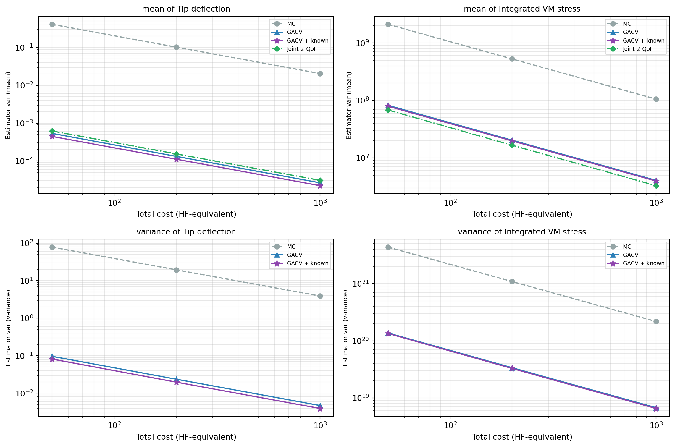
## Result 1: Variance vs Cost
The headline result (@fig-variance-vs-cost): group ACV with full subsets
delivers substantial variance reduction for **both the mean and the
variance** of each QoI. Exploiting the PCE's known statistics (mean or
variance) provides a further reduction — and for the mean, joint 2-QoI
estimation captures cross-QoI covariance for additional gain.
@fig-allocation shows the optimized sample allocation at a fixed budget.
```{python}
#| echo: false
#| fig-cap: "Predicted estimator variance vs total cost for the mean (top) and variance (bottom) of each QoI. MC baseline (dashed), group ACV with full subsets (blue), with known statistics (purple), and joint 2-QoI mean estimation (green, top row only)."
#| label: fig-variance-vs-cost
import matplotlib.pyplot as plt
from pyapprox_tutorials.figures._aerospace_beam import (
plot_variance_vs_cost_grid,
)
fig, axes = plt.subplots(2, 2, figsize=(12, 8))
plot_variance_vs_cost_grid(
axes, all_results, target_costs, qoi_names,
stat_names=["mean", "variance"],
)
fig.tight_layout()
plt.show()
```
The improvement from known statistics is modest here because the PCE
surrogate is nearly free to evaluate ($\sim 10^{-5}$ of the HF cost).
When the mean is known, far fewer samples are allocated to the PCE —
but those freed samples release very little budget since each PCE
evaluation costs almost nothing. As the evaluation cost of the surrogate
grows (larger PCE basis, neural network emulator, GP posterior), so too
will the gap between known and unknown.
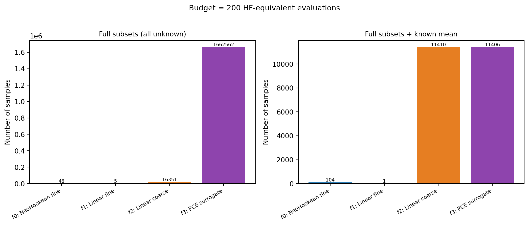
## Result 2: Where the Budget Goes
Comparing the sample allocations with and without the known mean
(@fig-allocation) shows **why** exploiting known statistics helps: when the
surrogate's mean is known analytically, the optimizer no longer needs to
spend samples estimating it. Those freed samples are redistributed to the
HF model, tightening the control-variate correction and lowering the
estimator variance — even though the total budget is unchanged.
```{python}
#| echo: false
#| fig-cap: "Optimized group ACV sample allocation at a fixed budget, without (left) and with (right) the PCE surrogate's known mean. When the surrogate mean is known, the optimizer redistributes samples from the surrogate to the HF model, tightening the control-variate correction."
#| label: fig-allocation
from pyapprox_tutorials.figures._aerospace_beam import plot_allocation_bars
mid_budget = target_costs[1]
# All-unknown allocation
est_unknown = GroupACVEstimatorIS(stat, costs, model_subsets=full_subsets)
alloc_unknown = GroupACVAllocationOptimizer(
est_unknown, optimizer=optimizer,
problem_config=log_ineq,
)
res_unknown = alloc_unknown.optimize(mid_budget, min_nhf_samples=2)
# Known-mean allocation
est_known = GroupACVEstimatorIS(
stat, costs, model_subsets=full_subsets,
known_quantities=known_quantities,
)
alloc_known = GroupACVAllocationOptimizer(
est_known, optimizer=optimizer,
problem_config=log_ineq,
)
res_known = alloc_known.optimize(mid_budget, min_nhf_samples=2)
fig, axes = plt.subplots(1, 2, figsize=(11, 4.5))
plot_allocation_bars(
axes[0], bkd.to_numpy(res_unknown.nsamples_per_model),
ensemble.model_names(), title="Full subsets (all unknown)",
)
plot_allocation_bars(
axes[1], bkd.to_numpy(res_known.nsamples_per_model),
ensemble.model_names(), title="Full subsets + known mean",
)
fig.suptitle(f"Budget = {mid_budget:.0f} HF-equivalent evaluations",
fontsize=11, y=1.02)
fig.tight_layout()
plt.show()
```
## Key Takeaways
- The beam *models* exist, but a multi-fidelity *problem* — shared
parameterization, random load, costs, pilot covariance, and a known-mean
surrogate — must be assembled
- The ensemble is partially ordered on purpose: a clean mesh-refinement pair, a
load-dependent physics pair, and a not-comparable surrogate — the case that
needs group ACV
- The headline variance-vs-cost result is predicted from the pilot covariance and
needs no closed-form truth
- A known-mean PCE surrogate enters as a mixed-known model and strictly lowers the
variance — the bridge to the surrogate-modeling tutorials
- Deflection and stress are estimated jointly with multi-output group ACV
## Exercises
1. Sweep `NPILOT` and plot the predicted group ACV variance at fixed budget vs
pilot size. How large a pilot stabilizes the allocation?
2. Drop the surrogate (model 3). How much does the group ACV variance rise at
fixed budget?
3. Raise the load distribution's mean so the nonlinear response stiffens. Watch
$\rho(f_0, f_1)$ fall and the optimizer shift samples away from the linear
fine model.
4. Replace the coarse linear model with an even coarser mesh. Does the extra cheap
model help, given its lower correlation?
## Next Steps
- [Group ACV Mixed Concept](group_acv_mixed_concept.qmd) — theory behind the
known-mean surrogate result
- [Pilot Studies](pilot_studies_concept.qmd) — sizing the pilot
- [Multi-Output ACV](multioutput_acv_concept.qmd) — the joint-QoI extension
- [Multi-Fidelity Estimation Cookbook](multifidelity_estimation_cookbook.qmd) —
the API this tutorial applies
## References
- [GJE2024] A. Gorodetsky, J. Jakeman, M. Eldred. *Grouped approximate control
variate estimators.* arXiv:2402.14736, 2024.
- [GGEJJCP2020] A. Gorodetsky, S. Geraci, M. Eldred, J. Jakeman. *A generalized
approximate control variate framework for multifidelity uncertainty
quantification.* Journal of Computational Physics, 408:109257, 2020.