
Control Variate Monte Carlo
PyApprox Tutorial Library
Reducing Monte Carlo estimator variance using a correlated low-fidelity model with a known statistic.
TipDownload Notebook
Learning Objectives
After completing this tutorial, you will be able to:
- Explain why a correlated low-fidelity model can reduce the variance of a Monte Carlo (MC) estimator
- Write down the Control Variate Monte Carlo (CVMC) estimator and identify its free parameter \(\eta\)
- State the optimal \(\eta\) and the resulting variance reduction in terms of model correlation
- Identify when CVMC helps and when it does not
Prerequisites
Complete Monte Carlo Sampling and Estimator Accuracy and MSE before this tutorial.
Motivation
The Estimator Accuracy tutorial showed that the variance of the MC mean estimator is \(\sigma^2_\alpha / N\), where \(\sigma^2_\alpha\) is the variance of the high-fidelity model output \(f_\alpha\) and \(N\) is the number of samples. Reducing this variance requires either more samples — which is expensive — or a smarter estimator.
Control Variate Monte Carlo (CVMC) is the simplest example of a smarter estimator. The idea: if we have access to a cheap model \(f_\kappa\) that is correlated with \(f_\alpha\) and whose mean \(\mu_\kappa = \mathbb{E}_\theta[f_\kappa(\boldsymbol{\theta})]\) is known exactly, we can use the cheap model to cancel a large fraction of the MC error.
Figure 1 illustrates this with two models of a 2D input. The surface plots show that \(f_\alpha\) and \(f_\kappa\) have similar shape — when one is large, so is the other. The scatter plot on the right confirms that model outputs are tightly correlated (\(\rho \approx 0.9\)).
The CVMC Estimator
The standard MC estimator of \(\mu_\alpha = \mathbb{E}_\theta[f_\alpha(\boldsymbol{\theta})]\) is
\[ \hat{\mu}_\alpha = \frac{1}{N} \sum_{k=1}^{N} f_\alpha(\boldsymbol{\theta}^{(k)}). \]
The CVMC estimator adds a correction term built from \(f_\kappa\):
\[ \hat{\mu}_\alpha^{\text{CV}} = \hat{\mu}_\alpha + \eta \left( \hat{\mu}_\kappa - \mu_\kappa \right) \tag{1}\]
where \(\hat{\mu}_\kappa = \frac{1}{N}\sum_{k=1}^N f_\kappa(\boldsymbol{\theta}^{(k)})\) is the MC mean of the low-fidelity model evaluated on the same \(N\) samples, and \(\eta\) is a scalar weight we are free to choose.
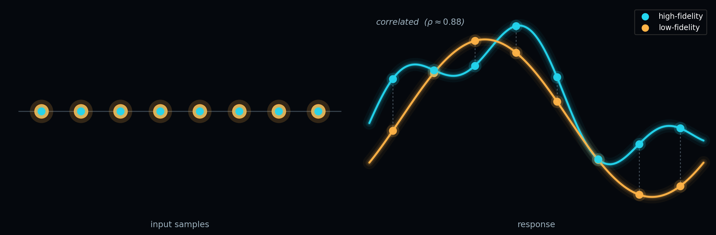
A critical feature of CVMC is that both models are evaluated at exactly the same set of input samples. Figure 2 illustrates this: on the left, every input sample (orange ring) has a high-fidelity evaluation (cyan dot) overlaid on top of it. On the right, the response curves show that the two models move together at these shared sample locations — the dashed connectors pair HF and LF values to highlight the correlation that the correction term exploits.
The correction term \(\hat{\mu}_\kappa - \mu_\kappa\) has mean zero — it is pure MC error in the low-fidelity estimate. Adding it to \(\hat{\mu}_\alpha\) does not introduce bias. But if the errors in \(\hat{\mu}_\alpha\) and \(\hat{\mu}_\kappa\) are correlated, choosing \(\eta\) with the right sign causes the correction to partially cancel the error in \(\hat{\mu}_\alpha\).
Variance Reduction Depends on Correlation
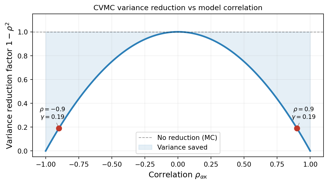
The key result (derived in Control Variate Analysis) is that with the optimal choice of \(\eta\), the CVMC estimator variance satisfies
\[ \mathbb{V}[\hat{\mu}_\alpha^{\text{CV}}] = \mathbb{V}[\hat{\mu}_\alpha] \left(1 - \rho^2_{\alpha\kappa}\right) \tag{2}\]
where \(\rho_{\alpha\kappa} = \mathrm{Corr}(f_\alpha, f_\kappa)\) is the correlation between the two model outputs. The factor \((1 - \rho^2_{\alpha\kappa})\) is always between 0 and 1, so CVMC always reduces (or at worst equals) the MC variance.
Figure 3 shows this relationship. Near-perfectly correlated models (\(|\rho| \approx 1\)) can reduce variance by orders of magnitude; uncorrelated models (\(\rho \approx 0\)) offer no benefit.
What CVMC Looks Like in Practice
Figure 4 shows the distribution of 1000 independent MC and CVMC mean estimates for a pair of models with \(\rho \approx 0.9\). Both estimators are centered on the true mean, confirming that CVMC is unbiased. But the CVMC histogram is dramatically narrower.

The Allocation Problem
Every multi-fidelity estimator faces the same core problem: given a computational budget \(P\), choose the free parameters of the estimator to minimize its variance. In the general case this takes the form
\[ \min_{\boldsymbol{\theta}} \;\mathbb{V}[\hat{\mu}(\boldsymbol{\theta})] \quad \text{subject to} \quad \mathrm{Cost}(\boldsymbol{\theta}) \leq P, \tag{3}\]
where \(\boldsymbol{\theta}\) collects all tunable parameters — sample counts, weights, and any structural choices — and \(\mathrm{Cost}(\boldsymbol{\theta})\) is the total computational cost of evaluating the estimator.
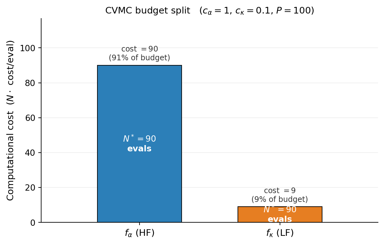
For CVMC the free parameters are the sample count \(N\) and the weight \(\eta\). Because both models are evaluated at every sample, the total cost is
\[ P = N\,(c_\alpha + c_\kappa), \tag{4}\]
where \(c_\alpha\) and \(c_\kappa\) are the per-sample costs of the two models. The optimal weight \(\eta^*\) is determined by the model covariance (see Control Variate Analysis) and does not depend on \(N\). The only remaining decision is \(N\) itself, and the budget constraint pins it directly:
\[ N^* = \left\lfloor \frac{P}{c_\alpha + c_\kappa} \right\rfloor. \tag{5}\]
There is no numerical optimization required — the allocation problem Equation 3 has a closed-form solution.
The closed form hides one feature worth seeing directly. Because both models are evaluated at the same \(N\) samples, the budget split between them is fixed entirely by their per-sample cost ratio \(c_\alpha : c_\kappa\) — there is no freedom to sample the cheap model more often. Figure 5 shows the consequence for an expensive high-fidelity model: at \(c_\alpha:c_\kappa = 10:1\) the high-fidelity evaluations consume roughly nine-tenths of the budget even though both models run the identical \(N^*\) times. This lock-step sampling is exactly the restriction that Approximate Control Variates relaxes by letting the low-fidelity model take additional samples of its own; however, this allocation is optimal for two models.
This is the simplest possible case. In the ACV estimator, the LF sample ratio \(r\) becomes a second free parameter and the allocation requires solving a one-dimensional optimization. In the many-model extensions and group ACV, the number of free parameters grows with the number of models and subsets, and the allocation becomes a high-dimensional constrained optimization problem.
When Does CVMC Help?
CVMC requires two ingredients:
A low-fidelity model \(f_\kappa\) with a known mean \(\mu_\kappa\). If \(\mu_\kappa\) is not known analytically, it must be estimated — introducing additional error. That case is handled by Approximate Control Variates.
High correlation \(|\rho_{\alpha\kappa}|\) between the models. The variance reduction \((1 - \rho^2)\) is only substantial when \(|\rho| \gtrsim 0.5\). A weakly correlated low-fidelity model offers little benefit.
The variance reduction is entirely due to cancellation of correlated errors, not a reduction in work — CVMC evaluates both models \(N\) times, at cost \(N(c_\alpha + c_\kappa)\) per Equation 4.
Key Takeaways
- CVMC adds a zero-mean correction \(\eta(\hat{\mu}_\kappa - \mu_\kappa)\) to the MC estimator; the correction is unbiased by construction
- With the optimal \(\eta\), the variance reduction factor is \((1 - \rho^2_{\alpha\kappa})\), determined entirely by the correlation between models
- \(|\rho| \approx 1\) gives near-perfect variance cancellation; \(\rho \approx 0\) gives no benefit
- CVMC requires \(\mu_\kappa\) to be known; when it is not, use Approximate Control Variates
Tip
Ready to try this? See API Cookbook → CVEstimator.
Exercises
If \(\rho = 0.7\), by what factor does CVMC reduce the variance compared to plain MC? How many fewer samples would you need to achieve the same standard error?
Suppose \(f_\kappa\) is the true model \(f_\alpha\) itself (i.e., \(\rho = 1\)). What does \(\hat{\mu}^{\text{CV}}_\alpha\) reduce to? Is this useful in practice?
The correction term is \(\eta(\hat{\mu}_\kappa - \mu_\kappa)\). Explain in words why a negative \(\eta\) is appropriate when the models are positively correlated (\(\rho > 0\)).
Next Steps
- Control Variate Analysis — Derive the optimal \(\eta\) and the \(1 - \rho^2\) result from first principles
- API Cookbook — Use the PyApprox CVMC API on a real model
- Approximate Control Variates — What to do when \(\mu_\kappa\) is unknown