import numpy as np
np.random.seed(42)
import matplotlib.pyplot as plt

from pyapprox.util.backends.numpy import NumpyBkd
from pyapprox.surrogates.kernels import ExponentialKernel
from pyapprox.surrogates.kle import MeshKLE

bkd = NumpyBkd()
rng = np.random.default_rng(42)

npts = 200
x = np.linspace(0, 2, npts)
# MeshKLE expects mesh_coords of shape (nphys_vars, ncoords)
mesh_coords = bkd.array(x[None, :])KLE I: Random Fields and the Karhunen-Loève Expansion
PyApprox Tutorial Library
Understand random fields, their covariance structure, and how the KLE decomposes them into deterministic spatial modes.
TipDownload Notebook
Learning Objectives
After completing this tutorial, you will be able to:
- Explain what a random field is and how its covariance kernel encodes spatial correlation
- Describe the Fredholm eigenvalue problem and the role of eigenfunctions and eigenvalues
- Use
MeshKLEwith anExponentialKernelto compute a KLE - Draw sample paths from the expansion and understand the effect of truncation
- Assess truncation error using eigenvalue decay and pointwise variance
A random field assigns a random variable to every point in space. The Karhunen-Loeve Expansion (KLE) decomposes it into deterministic spatial modes weighted by uncorrelated random scalars – a PCA for functions.
The covariance kernel controls spatial correlation
The covariance \(C(x, x') = \sigma^2 k(x, x')\) determines how similar the field is at nearby points. The correlation length \(\ell\) controls the spatial scale.
from pyapprox_tutorials.figures._kle import plot_cov_matrices

kernel_factory = lambda ell: ExponentialKernel(bkd.array([ell]), (0.01, 10.0), 1, bkd)

fig, axes = plt.subplots(1, 3, figsize=(12, 3.5), sharey=True)
plot_cov_matrices(mesh_coords, kernel_factory, [0.2, 0.5, 1.5], bkd, axes)
fig.suptitle("Covariance matrix $C(x,x')$ for three correlation lengths",
             fontsize=13)
plt.tight_layout()
plt.show()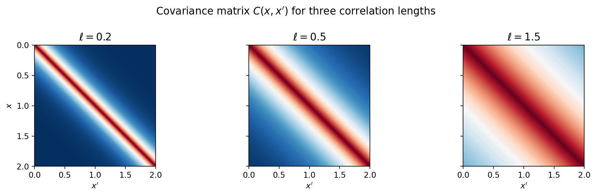
Larger \(\ell\) produces smoother fields with long-range dependence.
Eigenfunctions are the natural modes of the field
The Fredholm eigenvalue problem:
\[\int_D C(x, x')\,\phi_k(x')\,dx' = \lambda_k\,\phi_k(x)\]
gives eigenfunctions \(\phi_k\) (deterministic shapes) and eigenvalues \(\lambda_k\) (variance explained by each mode).
MeshKLE discretizes this integral using quadrature weights \(w_i\) and solves the weighted eigenproblem \(W^{1/2}\,C\,W^{1/2}\,\hat\phi = \lambda\,\hat\phi\).
from pyapprox_tutorials.figures._kle import plot_eigenvalues_eigenfunctions

# Trapezoid quadrature weights
dx = x[1] - x[0]
w = np.ones(npts) * dx
w[0] /= 2; w[-1] /= 2
quad_weights = bkd.array(w)

nterms = 6
ell = 0.5
kernel = ExponentialKernel(bkd.array([ell]), (0.01, 10.0), 1, bkd)
kle = MeshKLE(
    mesh_coords, kernel, sigma=1.0, nterms=nterms,
    quad_weights=quad_weights, bkd=bkd,
)

lam = bkd.to_numpy(kle.eigenvalues())
phi = bkd.to_numpy(kle.eigenvectors())

fig, axes = plt.subplots(1, 2, figsize=(12, 4))
plot_eigenvalues_eigenfunctions(x, lam, phi, nterms, axes[0], axes[1])
plt.tight_layout()
plt.show()
Eigenvalues decay – the field’s energy concentrates in the first few modes. The eigenfunctions are orthogonal spatial oscillations (analogous to Fourier modes but matched to the covariance structure).
The KLE: sample paths from random coefficients
\[f(x) = \mu(x) + \sum_{k=1}^{K} \sqrt{\lambda_k}\,\phi_k(x)\,z_k, \qquad z_k \sim \mathcal{N}(0,1)\]
Each draw of \(z_1, \ldots, z_K\) gives one realization of the random field. MeshKLE.__call__ evaluates this expansion: pass a (nterms, nsamples) coefficient array and get back (ncoords, nsamples) field values.
from pyapprox_tutorials.figures._kle import plot_sample_paths

K_list = [1, 2, 4, 6]
nsamples = 5
Z = rng.standard_normal((nterms, nsamples))

fields_list = []
for K in K_list:
    kle_K = MeshKLE(
        mesh_coords, kernel, sigma=1.0, nterms=K,
        quad_weights=quad_weights, bkd=bkd,
    )
    coef = bkd.array(Z[:K, :])
    fields_list.append(bkd.to_numpy(kle_K(coef)))

fig, axes = plt.subplots(1, len(K_list), figsize=(14, 3.8), sharey=True)
plot_sample_paths(x, fields_list, K_list, axes)
fig.suptitle("Sample paths using increasing numbers of KLE terms  "
             r"($\ell=0.5$, same $z_k$ draws)", fontsize=12)
plt.tight_layout()
plt.show()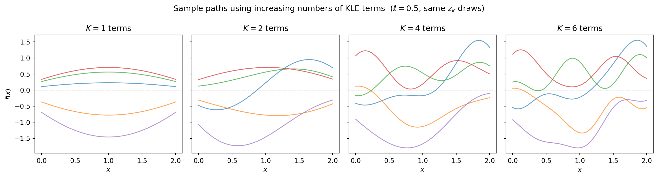
More terms produce rougher, more detailed realizations. With \(K = 6\) terms we have captured essentially all the variance for \(\ell = 0.5\).
Truncation error: how many terms do you need?
The fraction of variance explained by \(K\) terms is:
\[\frac{\sum_{k=1}^K \lambda_k}{\sum_{k=1}^{\infty} \lambda_k}\]
from pyapprox_tutorials.figures._kle import plot_kle_truncation_error

nterms_full = 100
kle_full = MeshKLE(
    mesh_coords, kernel, sigma=1.0, nterms=nterms_full,
    quad_weights=quad_weights, bkd=bkd,
)
lam_full = bkd.to_numpy(kle_full.eigenvalues())

kle_factory = lambda kern, nt: MeshKLE(
    mesh_coords, kern, sigma=1.0, nterms=nt,
    quad_weights=quad_weights, bkd=bkd,
)

fig, axes = plt.subplots(1, 2, figsize=(12, 4))
plot_kle_truncation_error(
    x, lam_full, nterms_full, mesh_coords, quad_weights,
    [0.2, 0.5, 1.5], bkd, kernel_factory, kle_factory,
    axes[0], axes[1],
)
plt.tight_layout()
plt.show()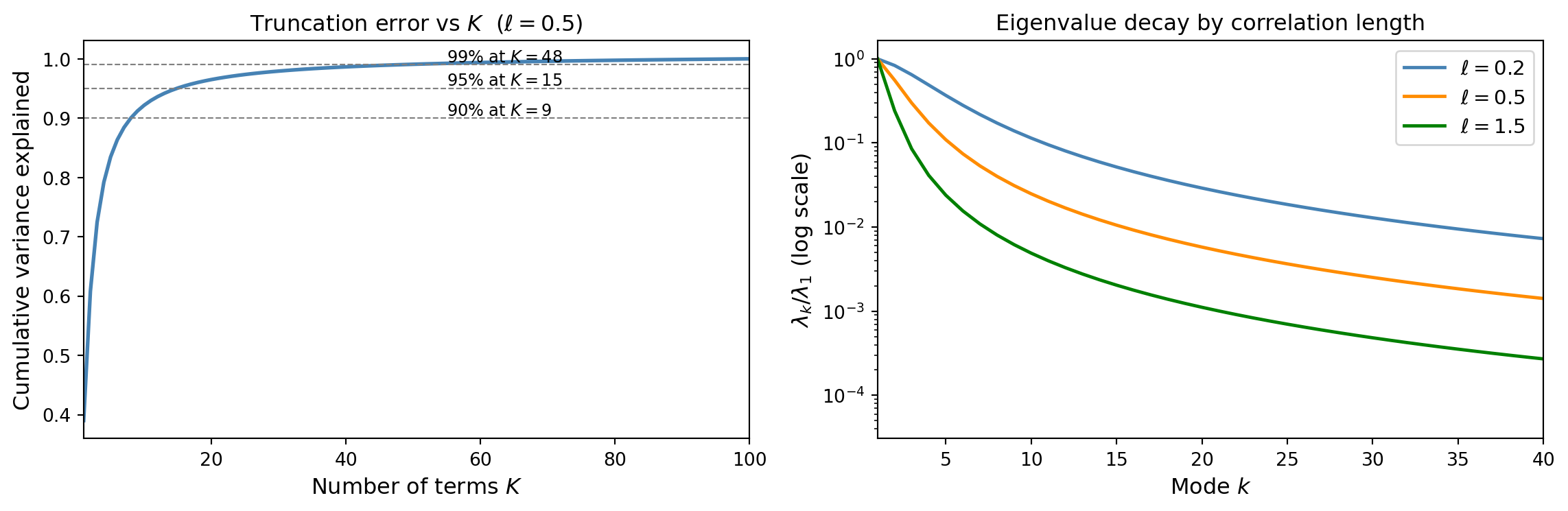
Key insight: larger \(\ell\) produces faster eigenvalue decay and fewer terms are needed. Smooth fields are cheap to represent; rough fields require many modes.
Pointwise variance: how much does truncation miss?
from pyapprox_tutorials.figures._kle import plot_pointwise_variance

K_vals = [1, 3, 6, 20]

# Exact variance (from full covariance diagonal)
C = bkd.to_numpy(kernel(mesh_coords, mesh_coords))
true_var = np.diag(C)

# Compute approximate variance for each truncation level
approx_vars = []
for K in K_vals:
    kle_K = MeshKLE(
        mesh_coords, kernel, sigma=1.0, nterms=K,
        quad_weights=quad_weights, bkd=bkd,
    )
    W = bkd.to_numpy(kle_K.weighted_eigenvectors())
    approx_vars.append(np.sum(W**2, axis=1))

fig, axes = plt.subplots(1, 2, figsize=(12, 4))
plot_pointwise_variance(x, true_var, K_vals, approx_vars, axes[0], axes[1])
plt.tight_layout()
plt.show()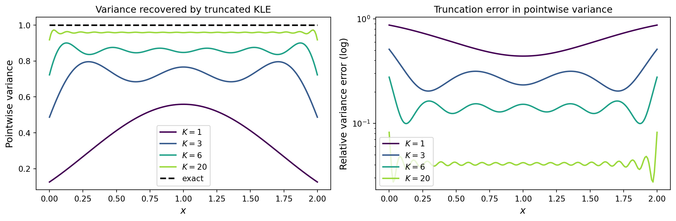
The boundary nodes recover more slowly – a systematic effect present in all mesh-based KLE methods (and worsened by boundary conditions in the SPDE approach).
Validation against the analytical solution
The exponential kernel on \([0, L]\) has known eigenvalues and eigenfunctions. AnalyticalExponentialKLE1D computes these analytically, providing a ground truth to validate the numerical MeshKLE solution.
from pyapprox.surrogates.kle import AnalyticalExponentialKLE1D
from pyapprox_tutorials.figures._kle import plot_analytical_validation

# Analytical solution for the same kernel on [0, 2]
kle_exact = AnalyticalExponentialKLE1D(
    corr_len=ell, sigma2=1.0, dom_len=2.0, nterms=nterms,
)
lam_exact = kle_exact.eigenvalues()

fig, axes = plt.subplots(1, 2, figsize=(12, 4))
plot_analytical_validation(lam, lam_exact, nterms, npts, axes[0], axes[1])
plt.tight_layout()
plt.show()
MeshKLE (blue) vs the analytical solution (orange) for the exponential kernel on \([0, 2]\). Right: relative eigenvalue error on a log scale, showing the numerical discretisation error decreases with mesh refinement.
The numerical eigenvalues from MeshKLE agree with the analytical solution to high accuracy. The error is controlled by the quadrature resolution – more mesh points would reduce it further.
Summary
| Concept | Meaning |
|---|---|
| Covariance kernel | Encodes spatial correlation structure |
| Eigenfunctions \(\phi_k\) | Deterministic spatial modes |
| Eigenvalues \(\lambda_k\) | Variance in each mode; must decay for KLE to be useful |
| KLE coefficients \(z_k\) | Independent \(\mathcal{N}(0,1)\) random variables |
| Truncation at \(K\) terms | Controls accuracy; larger \(\ell\) means fewer terms needed |
Next: KLE II shows how MeshKLE and DataDrivenKLE compute these eigenpairs from a kernel function or from data samples respectively.