import numpy as np
import matplotlib.pyplot as plt
from pyapprox.util.backends.numpy import NumpyBkd
from pyapprox_benchmarks.statest import PolynomialEnsembleBenchmark
from pyapprox.statest import MultiOutputMean, MFMCEstimator, MCEstimator
from pyapprox.statest.acv.allocation import default_allocator_factory
from pyapprox.statest.acv.base import FittedACVEstimator
from pyapprox.statest.allocation import MCAllocator

bkd = NumpyBkd()
np.random.seed(1)
benchmark = PolynomialEnsembleBenchmark(bkd, nmodels=3)
nmodels   = 3
nqoi      = 1
costs_v   = bkd.array([1.0, 0.1, 0.05])
costs_np  = bkd.to_numpy(costs_v)
prior     = benchmark.problem().prior()
models    = benchmark.problem().models()
true_mean = float(bkd.to_numpy(benchmark.ensemble_means())[0, 0])

cov_oracle  = benchmark.ensemble_covariance()
oracle_stat = MultiOutputMean(nqoi, bkd)
oracle_stat.set_pilot_quantities(cov_oracle)Pilot Studies: Analysis
PyApprox Tutorial Library
Decomposing the MSE of a pilot-based ACV estimator into allocation error and budget depletion, deriving the optimal pilot fraction, and quantifying sensitivity to pilot size as a function of model correlation and total budget.
TipDownload Notebook
Learning Objectives
After completing this tutorial, you will be able to:
- Decompose the MSE of a pilot-based estimator into variance (from budget depletion) and bias-squared (from allocation error)
- Describe how the optimal pilot fraction \(f^* = P_p / P\) depends on budget, correlation, and number of models
- Show numerically that the optimal \(N_p\) shifts with total budget \(P\) and model correlation \(\rho\)
- Quantify the covariance estimation error as a function of \(N_p\) using the Wishart distribution result
- Design a pilot study for a new problem given a budget, model count, and target MSE
Prerequisites
Complete Pilot Studies Concept and General ACV Analysis before this tutorial.
Setup
MSE Decomposition
The MSE of a pilot-based ACV estimator \(\hat{\mu}_0^{\text{ACV}}(N_p, P)\) decomposes as:
\[ \text{MSE}(\hat{\mu}_0) = \underbrace{\mathbb{V}[\hat{\mu}_0 \mid \hat{\boldsymbol{\Sigma}}]}_{\text{estimator variance given allocation}} + \underbrace{\left(\mathbb{E}[\hat{\mu}_0] - \mu_0\right)^2}_{\text{bias}^2}, \]
where the expectation is over both the pilot samples and the main estimator samples.
Estimator variance is the variance of \(\hat{\mu}_0\) at the allocation determined by \(\hat{\boldsymbol{\Sigma}}\). When \(\hat{\boldsymbol{\Sigma}} \approx \boldsymbol{\Sigma}\), this is close to the oracle variance. When \(\hat{\boldsymbol{\Sigma}}\) is noisy, the chosen allocation is suboptimal and the variance is higher.
Bias arises because the control variate coefficient \(\hat{\alpha} = -\hat{\sigma}_{0,1}/\hat{\sigma}_{1,1}\) is a ratio of random variables. For finite \(N_p\), \(\mathbb{E}[\hat{\alpha}] \neq \alpha^*\), introducing a small residual bias. The bias vanishes as \(N_p \to \infty\).
In practice, the bias contribution is small compared to the variance contribution unless \(N_p\) is very small (\(< M+2\)). The dominant effect is the allocation error from a noisy \(\hat{\boldsymbol{\Sigma}}\).
P_total   = 100.0
ntrials   = 600
npilot_list = [5, 8, 12, 20, 35, 60, 80]

def run_pilot_trial(seed, npilot, budget):
    np.random.seed(seed)
    s_p = prior.rvs(npilot)
    vals_p = [m(s_p) for m in models]
    stat = MultiOutputMean(nqoi, bkd)
    (cov_hat,) = stat.compute_pilot_quantities(vals_p)
    stat.set_pilot_quantities(cov_hat)
    est = MFMCEstimator(stat, costs_v)
    try:
        alloc_result = default_allocator_factory(est).allocate(budget)
        fitted = FittedACVEstimator(est, alloc_result)
        np.random.seed(seed + 1000)
        s_main = fitted.generate_samples_per_model(prior.rvs)
        vals_main = [m(s) for m, s in zip(models, s_main)]
        return float(fitted(vals_main))
    except Exception:
        return float("nan")

oracle_est = MFMCEstimator(oracle_stat, costs_v)
oracle_fitted = FittedACVEstimator(
    oracle_est, default_allocator_factory(oracle_est).allocate(P_total))
oracle_var = float(bkd.to_numpy(oracle_fitted.covariance())[0, 0])
mc_est_tmp = MCEstimator(oracle_stat, costs_v[:1])
mc_fitted_tmp = MCAllocator(mc_est_tmp).allocate(P_total)
mc_var     = float(bkd.to_numpy(mc_fitted_tmp.covariance())[0, 0])

mse_vals, var_vals, bias2_vals = [], [], []
for npilot in npilot_list:
    pilot_cost  = costs_np.sum() * npilot
    budget_main = P_total - pilot_cost
    estimates   = np.array([run_pilot_trial(s, npilot, budget_main)
                            for s in range(ntrials)])
    mse  = np.mean((estimates - true_mean)**2)
    var_ = np.var(estimates)
    b2   = (np.mean(estimates) - true_mean)**2
    mse_vals.append(mse);  var_vals.append(var_);  bias2_vals.append(b2)

oracle_est2 = MFMCEstimator(oracle_stat, costs_v)
oracle_fitted2 = FittedACVEstimator(
    oracle_est2, default_allocator_factory(oracle_est2).allocate(P_total))
oracle_var = float(bkd.to_numpy(oracle_fitted2.covariance())[0, 0])

fig, ax = plt.subplots(figsize=(9, 4.5))
ax.plot(npilot_list, [m/mc_var for m in mse_vals],   "-o", color="#2C7FB8",
        lw=2.2, ms=7, label="Total MSE")
ax.plot(npilot_list, [v/mc_var for v in var_vals],   "-s", color="#27AE60",
        lw=1.8, ms=6, label="Variance component")
ax.plot(npilot_list, [b/mc_var for b in bias2_vals], "-^", color="#E67E22",
        lw=1.8, ms=6, label="Bias² component")
ax.axhline(oracle_var/mc_var, color="k", ls="--", lw=1.8,
           label=f"Oracle ACV ({oracle_var/mc_var:.3f})")
ax.axhline(1.0, color="#c0392b", ls=":", lw=1.5, label="MC baseline")
ax.set_xlabel("Pilot samples $N_p$", fontsize=11)
ax.set_ylabel("Component / MC MSE", fontsize=11)
ax.set_title("MSE decomposition — MFMC, P=100, pilot cost deducted", fontsize=11)
ax.legend(fontsize=9)
ax.grid(True, alpha=0.2)
ax.set_ylim(bottom=0)
plt.tight_layout()
plt.show()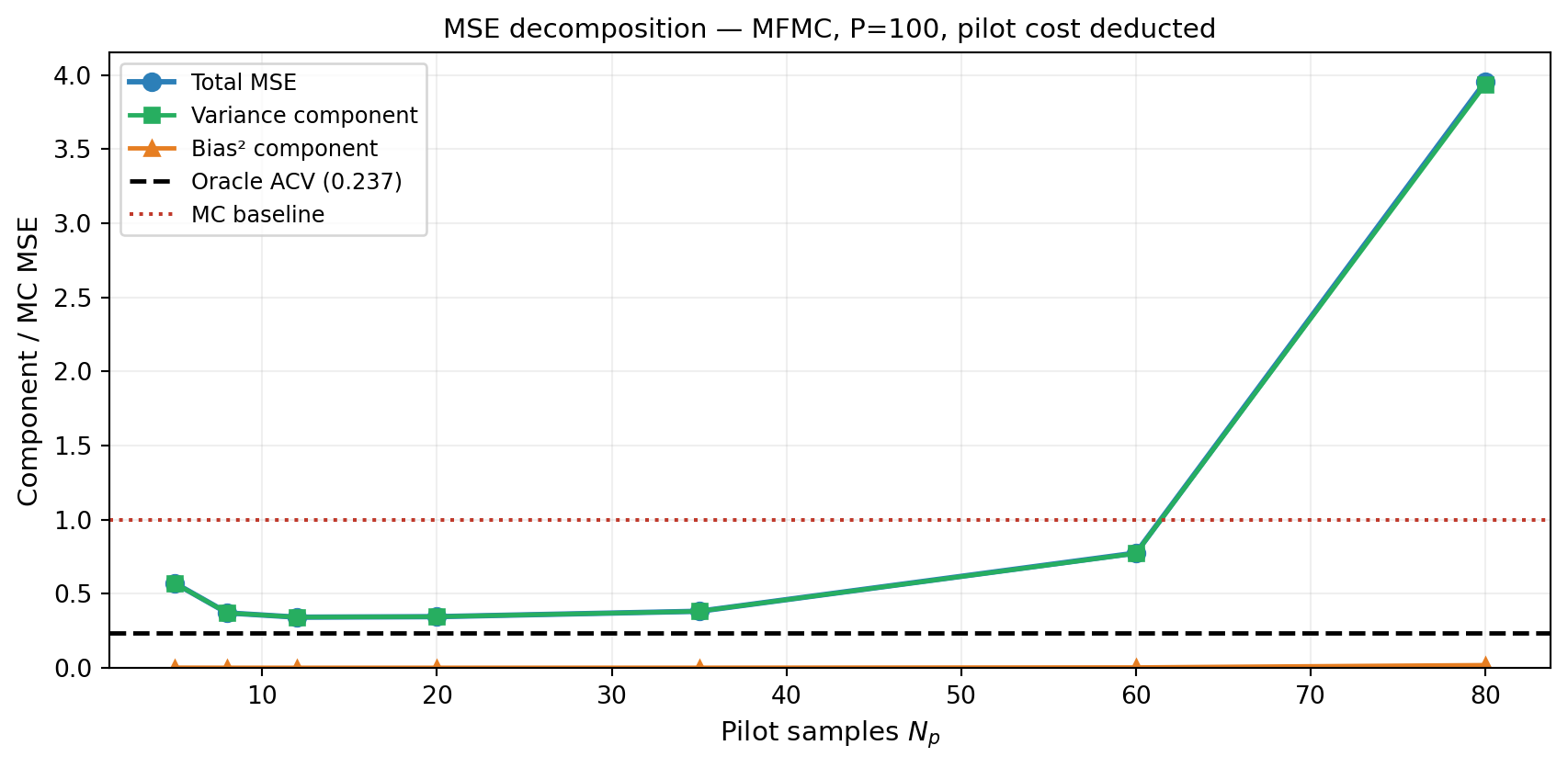
Sensitivity to Total Budget
The optimal pilot fraction \(f^* = N_p^* \sum_\alpha C_\alpha / P\) is not fixed — it depends on the total budget \(P\). At small \(P\), covariance estimation matters less (the estimator is dominated by HF sample count), so a smaller fraction is optimal. At large \(P\), a precise covariance estimate is worth more.
budgets   = [100.0, 300.0, 500.0]
cols      = ["#8E44AD", "#2C7FB8", "#27AE60"]
npilot_grids = {
    100.0: [5, 8, 12, 20, 35, 60, 80],
    300.0: [5, 10, 20, 40, 80, 150, 250],
    500.0: [10, 20, 40, 80, 160, 250, 350],
}
ntrials_b = 300

fig, ax = plt.subplots(figsize=(10, 4.5))
for P, col in zip(budgets, cols):
    oracle_est_b = MFMCEstimator(oracle_stat, costs_v)
    oracle_fitted_b = FittedACVEstimator(
        oracle_est_b, default_allocator_factory(oracle_est_b).allocate(P))
    oracle_var_b = float(bkd.to_numpy(oracle_fitted_b.covariance())[0, 0])
    mc_est_b     = MCEstimator(oracle_stat, costs_v[:1])
    mc_fitted_b  = MCAllocator(mc_est_b).allocate(P)
    mc_var_b     = float(bkd.to_numpy(mc_fitted_b.covariance())[0, 0])

    mse_b = []
    for npilot in npilot_grids[P]:
        pilot_cost   = costs_np.sum() * npilot
        budget_main  = P - pilot_cost
        estimates_b  = np.array([run_pilot_trial(s, npilot, budget_main)
                                 for s in range(ntrials_b)])
        mse_b.append(float(np.mean((estimates_b - true_mean)**2)) / mc_var_b)

    grid = npilot_grids[P]
    best_i = int(np.argmin(mse_b))
    ax.plot(grid, mse_b, "-o", color=col, lw=2, ms=6, label=f"P={int(P)}")
    ax.plot(grid[best_i], mse_b[best_i], "*", color=col, ms=14,
            markeredgecolor="k", markeredgewidth=0.8, zorder=5)
    ax.axhline(oracle_var_b / mc_var_b, color=col, ls=":", lw=1, alpha=0.5)

ax.set_xlabel("Pilot samples $N_p$", fontsize=11)
ax.set_ylabel("MSE / MC MSE", fontsize=11)
ax.set_title("Optimal pilot size shifts with total budget (★ = optimum)", fontsize=11)
ax.legend(fontsize=9)
ax.grid(True, alpha=0.2)
plt.tight_layout()
plt.show()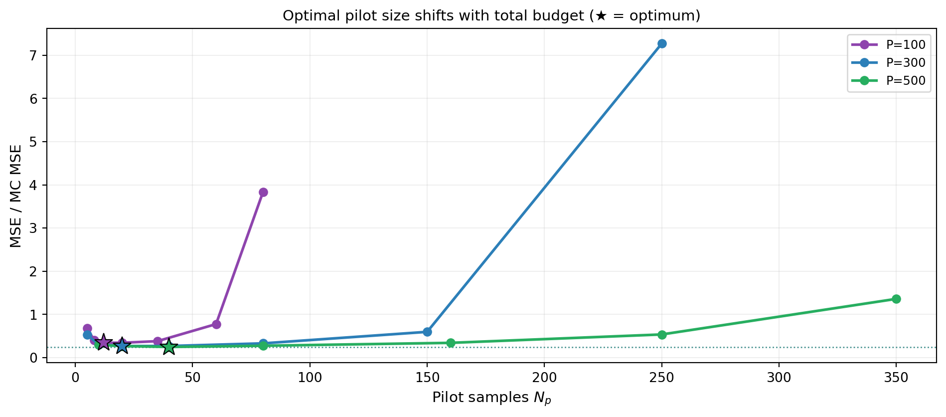
Sensitivity to Model Correlation
Weakly-correlated models require larger pilot studies because the relevant off-diagonal covariance entries are harder to estimate from finite samples.
from pyapprox_benchmarks.statest import TunableEnsembleBenchmark

# theta1 controls rho_01: larger theta1 → higher correlation
theta_vals = [1.4, 1.0, 0.6]
cols_rho   = ["#2C7FB8", "#27AE60", "#E67E22"]
npilot_grid_rho = [5, 8, 12, 20, 35, 60, 80]
ntrials_r = 300

fig, ax = plt.subplots(figsize=(9, 4.5))

for theta1, col in zip(theta_vals, cols_rho):
    bm = TunableEnsembleBenchmark(bkd, theta1=theta1)
    bm_models = bm.problem().models()
    bm_prior  = bm.problem().prior()
    bm_costs  = bm.problem().costs()
    bm_cov    = bm.ensemble_covariance()
    bm_mean   = float(bkd.to_numpy(bm.ensemble_means())[0, 0])
    nmod      = bm.problem().nmodels()
    costs_np_bm = bkd.to_numpy(bm_costs)

    # Compute correlation for label
    cov_np_bm = bkd.to_numpy(bm_cov)
    rho01 = cov_np_bm[0, 1] / np.sqrt(cov_np_bm[0, 0] * cov_np_bm[1, 1])

    # Oracle and MC baselines
    stat_o = MultiOutputMean(1, bkd)
    stat_o.set_pilot_quantities(bm_cov)
    oracle_e = MFMCEstimator(stat_o, bm_costs)
    oracle_fitted_e = FittedACVEstimator(
        oracle_e, default_allocator_factory(oracle_e).allocate(100.0))
    oracle_var = float(bkd.to_numpy(oracle_fitted_e.covariance())[0, 0])
    mc_e = MCEstimator(stat_o, bm_costs[:1])
    mc_fitted_e = MCAllocator(mc_e).allocate(100.0)
    mc_var = float(bkd.to_numpy(mc_fitted_e.covariance())[0, 0])

    def run_trial(seed, npilot, budget,
                  _models=bm_models, _prior=bm_prior, _costs=bm_costs,
                  _nmod=nmod, _mean=bm_mean):
        np.random.seed(seed)
        s_p = _prior.rvs(npilot)
        vals_p = [m(s_p) for m in _models]
        stat_t = MultiOutputMean(1, bkd)
        (cov_hat,) = stat_t.compute_pilot_quantities(vals_p)
        stat_t.set_pilot_quantities(cov_hat)
        est = MFMCEstimator(stat_t, _costs)
        try:
            alloc_result = default_allocator_factory(est).allocate(budget)
            fitted = FittedACVEstimator(est, alloc_result)
            np.random.seed(seed + 2000)
            spm = fitted.generate_samples_per_model(_prior.rvs)
            vpm = [_models[a](spm[a]) for a in range(_nmod)]
            return float(fitted(vpm))
        except Exception:
            return float("nan")

    mse_r = []
    for npilot in npilot_grid_rho:
        budget_main = 100.0 - costs_np_bm.sum() * npilot
        ests_r = np.array([run_trial(s, npilot, budget_main)
                           for s in range(ntrials_r)])
        ests_r = ests_r[np.isfinite(ests_r)]
        mse_r.append(float(np.mean((ests_r - bm_mean)**2)) / mc_var)

    ax.plot(npilot_grid_rho, mse_r, "-o", color=col, lw=2.2, ms=6,
            label=f"$\\rho_{{01}}={rho01:.2f}$")
    ax.axhline(oracle_var / mc_var, color=col, ls=":", lw=1.2, alpha=0.5,
               label=f"Oracle $\\rho_{{01}}={rho01:.2f}$")

ax.set_xlabel("Pilot samples $N_p$", fontsize=11)
ax.set_ylabel("MSE / MC MSE", fontsize=11)
ax.set_title("Pilot sensitivity vs model correlation  (P=100, pilot cost deducted)", fontsize=11)
ax.legend(fontsize=9)
ax.grid(True, alpha=0.2)
plt.tight_layout()
plt.show()
Figure 3 uses the tunable_ensemble_3model benchmark with three values of \(\theta_1\) to produce different HF–MF correlations.
Key Takeaways
- The MSE of a pilot-based estimator decomposes into a variance term (dominant, from allocation error) and a bias² term (negligible except for very small \(N_p\))
- The optimal pilot size \(N_p^*\) increases with total budget \(P\) and decreases with model correlation \(\rho\) (see Figure 2, Figure 3)
- For \(\rho \geq 0.9\), \(N_p = 10\)–\(20\) is typically sufficient at moderate budgets
- For \(\rho < 0.7\), consider whether including the model is beneficial at all before investing in a larger pilot (see Ensemble Selection)
Exercises
From Figure 1, at what \(N_p\) does the total MSE first fall below \(1.1\times\) the oracle ACV MSE? Is this the same as the MSE-minimum point?
From Figure 3, at which \(N_p\) does each correlation level first drop below the MC baseline? How does this crossover point depend on \(\rho_{01}\)?
From Figure 2, does the optimal pilot fraction \(N_p^*/P\) increase or decrease as \(P\) grows? Is this consistent with the intuition that a larger budget makes a precise covariance estimate more valuable?