import numpy as np
import matplotlib.pyplot as plt
from pyapprox.util.backends.numpy import NumpyBkd
from pyapprox_benchmarks.expdesign.linear_gaussian import (
    build_linear_gaussian_kl_benchmark,
)
from pyapprox.expdesign.objective import create_kl_oed_objective_from_data
from pyapprox.expdesign.quadrature import HaltonSampler
from pyapprox.expdesign.quadrature.oed import build_oed_joint_distribution
from pyapprox.probability.joint import IndependentJoint
from pyapprox.probability.univariate import GaussianMarginalBayesian OED: MC vs. Halton for EIG Estimation
PyApprox Tutorial Library
Why randomly-shifted Halton sequences reduce MSE compared to i.i.d. Monte Carlo for the double-loop EIG estimator, and when QMC stops helping.
TipDownload Notebook
Learning Objectives
After completing this tutorial, you will be able to:
- Explain why stratified low-discrepancy sequences reduce estimator variance compared to i.i.d. Monte Carlo
- Implement a randomly-shifted Halton sequence and use it as a drop-in replacement for the outer loop draws
- Measure the empirical MSE for MC and Halton and confirm that Halton achieves lower MSE for the same sample count
- Identify the conditions (smoothness, dimensionality) under which QMC helps
Prerequisites
Complete Verifying Convergence before this tutorial, where we established that the outer sample count \(M\) drives variance at rate \(O(1/M)\). Here we ask: can we reduce the constant in front of \(O(1/M)\) by sampling more carefully?
Why QMC?
Standard Monte Carlo draws i.i.d. uniform points, which cluster and leave gaps by chance. The estimator variance is \(O(1/M)\) regardless of the dimension \(D+K\) or the smoothness of the integrand.
Quasi-Monte Carlo (QMC) replaces i.i.d. draws with a deterministic low-discrepancy sequence that fills space more evenly. For smooth integrands, the Koksma–Hlawka inequality guarantees an error bound of \(O\!\left((\log M)^{D+K} / M\right)\). The exponent on \(M\) is the same as standard MC, but the more uniform coverage reduces the constant in front, giving lower MSE at every sample count.
Randomized QMC (RQMC) adds a uniform random shift to the Halton sequence before mapping to the normal distribution. The shift preserves the low-discrepancy structure while making each realization an unbiased estimator of EIG — so we can still compute MSE across multiple RQMC realizations.
NoteWhy the outer loop specifically?
QMC targets the outer \(M\) samples because that is where the \(O(1/M)\) variance lives. The inner \(N_\text{in}\) samples control bias, which is a different error source. Replacing the inner loop with QMC gives a smaller gain and is harder to analyse theoretically.
Setup
We use the same linear Gaussian model as in earlier tutorials — a degree-2 polynomial basis with 5 sensors — so results are directly comparable to the convergence plots in Verifying Convergence.
bkd = NumpyBkd()

nobs, degree, noise_std, prior_std = 5, 2, 0.5, 0.5
benchmark = build_linear_gaussian_kl_benchmark(nobs, degree, noise_std, prior_std, bkd)
K = benchmark.problem().nobs()      # 5 sensors
D = benchmark.problem().nparams()   # 3 parameters
obs_map = benchmark.problem().obs_map()

weights = bkd.ones((K, 1)) / K   # uniform design weights
true_eig = benchmark.exact_eig(weights)
Halton Sequence
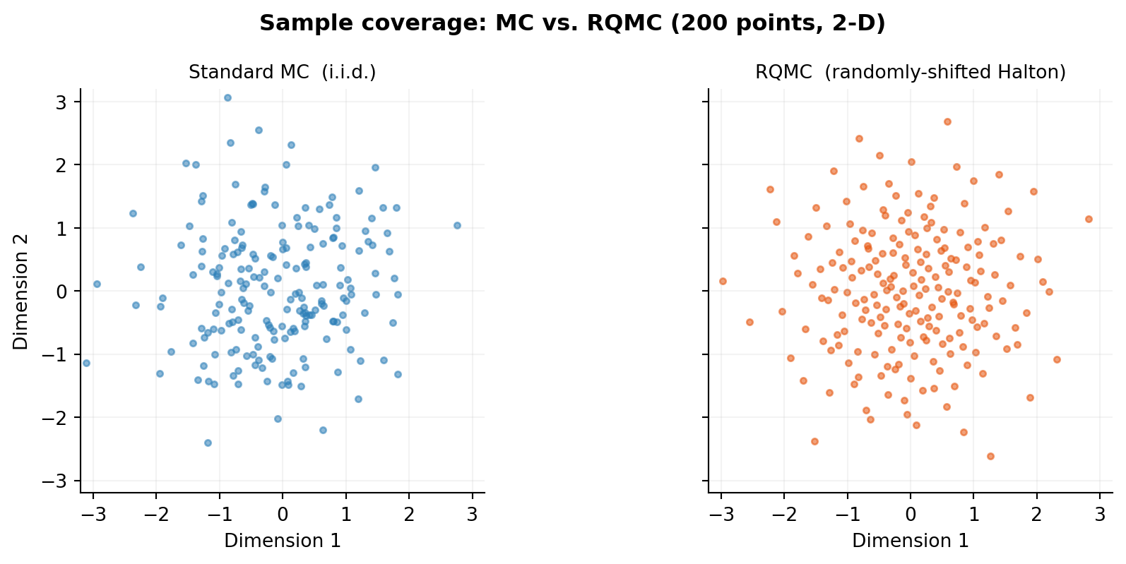
The Halton sequence in dimension \(d\) uses the \(d\)-th prime as its base, producing a sequence that fills \([0,1]^d\) far more evenly than uniform random draws. HaltonSampler (backed by scipy.stats.qmc) handles scrambling, random shifting, and inverse-CDF transformation to any target distribution.
The figure below compares 200 points drawn by standard MC (left) vs. RQMC (right) for the first two dimensions (the \(\theta_1\) and \(\theta_2\) directions). The RQMC points tile the space without clusters or gaps.
EIG Estimator with RQMC Outer Loop
The double-loop EIG estimator is unchanged — we simply replace the i.i.d. outer draws with RQMC samples. The create_kl_oed_objective_from_data factory builds a KLOEDObjective from pre-computed forward model outputs and latent noise, so swapping MC for RQMC only changes how those arrays are generated.
noise_var = bkd.full((K,), noise_std**2)

# Build the joint prior+noise distribution for QMC sampling
joint_dist = build_oed_joint_distribution(benchmark.problem(), bkd)

def eig_from_samples(theta_out, latent, N_in, seed_inner):
    """
    EIG estimate from pre-drawn outer samples.

    theta_out : (D, M) — parameter samples (already in prior scale)
    latent    : (K, M) — noise samples (already in noise scale)
    """
    outer_shapes = obs_map(theta_out)                       # (K, M)

    np.random.seed(seed_inner)
    theta_in     = bkd.array(np.random.randn(D, N_in) * prior_std)
    inner_shapes = obs_map(theta_in)                        # (K, N_in)

    obj = create_kl_oed_objective_from_data(
        noise_var, outer_shapes, inner_shapes, latent, bkd,
    )
    return obj.expected_information_gain(weights)
Convergence Comparison
We measure MSE over N_rep=50 independent realizations at each sample count, using a shared inner MC seed to isolate the effect of the outer sampling strategy.
outer_counts = [50, 100, 200, 400, 800, 1600]
N_in         = 500     # large enough that inner bias is negligible
N_rep        = 50
dim          = D + K   # joint parameter + noise dimensionality

mse_mc  = []
mse_qmc = []

rng = np.random.default_rng(0)

for M in outer_counts:
    ests_mc, ests_qmc = [], []
    for s in range(N_rep):
        # MC outer draws: scale standard normal by prior_std / noise_std
        z_mc = rng.standard_normal((dim, M))
        theta_mc = bkd.array(z_mc[:D, :] * prior_std)
        latent_mc = bkd.array(z_mc[D:, :])
        ests_mc.append(eig_from_samples(theta_mc, latent_mc, N_in, seed_inner=1000+s))

        # RQMC outer draws via HaltonSampler with joint distribution
        halton = HaltonSampler(dim, bkd, distribution=joint_dist, seed=s)
        z_qmc, _ = halton.sample(M)   # (dim, M) — already in prior/noise scale
        theta_qmc = z_qmc[:D, :]
        latent_qmc = z_qmc[D:, :]
        ests_qmc.append(eig_from_samples(theta_qmc, latent_qmc, N_in, seed_inner=1000+s))

    mse_mc.append( np.mean((np.array(ests_mc)  - true_eig)**2))
    mse_qmc.append(np.mean((np.array(ests_qmc) - true_eig)**2))
slope_mc  = np.polyfit(np.log(outer_counts), np.log(mse_mc),  1)[0]
slope_qmc = np.polyfit(np.log(outer_counts), np.log(mse_qmc), 1)[0]
When Does QMC Help?
QMC improves convergence when the integrand is smooth. For the double-loop EIG estimator with Gaussian noise and a linear forward model, the integrand is smooth in all dimensions and the gain is reliable. In other settings:
- High dimension (\(D+K \gg 20\)): the \((\log M)^{D+K}\) factor in the theoretical bound grows large; QMC still helps empirically but the advantage narrows.
- Discontinuous integrands: the Koksma–Hlawka bound requires bounded variation; sharp discontinuities can eliminate the advantage.
- Inner loop: the inner loop evidence average has a \(\log\) applied; its integrand is smooth too, but since bias rather than variance is the target, RQMC inner draws give smaller gains per unit budget.
NoteQMC and the reparameterization trick
When using RQMC outer draws, the latent noise rows of outer_z (rows D:D+K) play the role of the stored \(\boldsymbol{\varepsilon}^{(m)}\) in the C3 gradient term. Because the RQMC points are drawn once per optimization step and held fixed, the reparameterization gradient formula applies unchanged — switching from MC to RQMC only changes how HaltonSampler generates the joint samples, not the KLOEDObjective.jacobian() computation.
Key Takeaways
- RQMC (randomly-shifted Halton) is a drop-in replacement for the outer MC draws that achieves lower MSE at no additional computational cost per sample.
- Both MC and RQMC converge at \(O(1/M)\) asymptotically, but RQMC has a smaller constant: the more uniform coverage reduces the variance at every sample count.
- The random shift is essential: it makes each realization an unbiased EIG estimator, preserving the ability to estimate MSE across realizations.
- RQMC targets the outer variance only; the inner bias is unaffected.
- The gain diminishes in very high dimensions or for non-smooth integrands.
Exercises
Create a
HaltonSamplerwithscramble=False(no random shift). How does the MSE change? Is the estimator still unbiased across realizations?Replace
HaltonSamplerwithSobolSampler(frompyapprox.expdesign.quadrature.sobol). Does it give a steeper slope than Halton for this problem?Fix \(M=400\) and plot MSE as a function of the inner sample count \(N_\text{in}\) for both MC and RQMC outer draws. Do the inner-loop bias curves differ between the two methods? Why or why not?
Try \(D=5\) parameters (set
degree=4). Does the RQMC advantage shrink relative to thedegree=2case? At what dimension do you expect the advantage to effectively disappear?
Next Steps
- Goal-Oriented Bayesian OED — when prediction accuracy matters more than parameter estimation
- Bayesian OED for Prediction: Convergence — analogous verification for the risk-aware utility