
Multi-Level Monte Carlo
PyApprox Tutorial Library
Estimating high-fidelity model statistics using a hierarchy of models by accumulating corrections between consecutive levels.
TipDownload Notebook
Learning Objectives
After completing this tutorial, you will be able to:
- Explain the telescoping identity that underpins the MLMC estimator
- Describe why estimating level differences rather than model outputs directly reduces variance
- State why MLMC sample sets are kept independent across levels
- Identify when MLMC is a good fit and when the level-difference variances will be small
Prerequisites
Complete Approximate Control Variates before this tutorial.
Motivation: Many Cheap Models, One Expensive Truth
The ACV tutorial showed how a single cheap model can reduce the variance of a HF MC estimator. What if we have not one but many models arranged in a hierarchy of increasing fidelity and cost? Multi-Level Monte Carlo (MLMC) [GOR2008] exploits such a hierarchy differently from ACV: rather than correcting the HF estimate, it decomposes the HF mean into a sum of level-wise corrections and estimates each correction cheaply at the level where it is cheapest to do so.
MLMC was originally developed for finite-element models where the levels correspond to successively refined meshes. The same idea applies to any sequence of models ordered by accuracy and cost.
The Telescoping Identity
Let \(f_0, f_1, \ldots, f_M\) be a hierarchy of models ordered by decreasing fidelity and cost (\(f_0\) is the expensive high-fidelity model, \(f_M\) is the cheapest). Define \(f_{M+1} \equiv 0\). Then
\[ \mathbb{E}[f_0] = \sum_{\ell=0}^{M} \mathbb{E}[f_\ell - f_{\ell+1}] \tag{1}\]
because the sum telescopes: all intermediate expectations cancel, leaving only \(\mathbb{E}[f_0] - \mathbb{E}[f_{M+1}] = \mathbb{E}[f_0]\).
Each term \(\mathbb{E}[f_\ell - f_{\ell+1}]\) is the expected correction from level \(\ell+1\) to level \(\ell\). This is the quantity MLMC estimates at each level.
Why Differences Have Small Variance
The variance of a correction \(f_\ell - f_{\ell+1}\) is small whenever \(f_\ell \approx f_{\ell+1}\) — that is, whenever consecutive models in the hierarchy are similar to each other. This is exactly what we expect from a well-designed model sequence: a fine mesh and the next-finer mesh produce nearly identical outputs, so their difference varies little across samples.
Figure 1 makes this concrete for a five-level polynomial hierarchy \(f_\ell(z) = z^{5-\ell}\), \(z \sim \mathcal{U}[0,1]\). The variance of each level’s correction \(Y_\ell = f_\ell - f_{\ell+1}\) decreases rapidly as \(\ell\) increases (moving toward cheaper models), while the cost per sample also decreases. The cheap levels concentrate most of the correction work at negligible expense.
The MLMC Estimator
MLMC estimates each term in Equation 1 using its own independent sample set \(\mathcal{Z}_\ell\) of size \(N_\ell\):
\[ \hat{\mu}_0^{\text{ML}} = \sum_{\ell=0}^{M} \hat{Y}_\ell, \qquad \hat{Y}_\ell = \frac{1}{N_\ell} \sum_{k=1}^{N_\ell} \bigl(f_\ell(\boldsymbol{\theta}^{(k)}) - f_{\ell+1}(\boldsymbol{\theta}^{(k)})\bigr). \tag{2}\]
Because the sample sets are independent across levels, the estimator variance is simply
\[ \mathbb{V}[\hat{\mu}_0^{\text{ML}}] = \sum_{\ell=0}^{M} \frac{\mathbb{V}[Y_\ell]}{N_\ell}. \tag{3}\]
We can make each term small by choosing \(N_\ell\) large, but \(N_\ell\) only needs to be large when \(\mathbb{V}[Y_\ell]\) is large — which is exactly at the expensive levels near \(\ell = 0\). The cheap levels (\(\ell\) near \(M\)) have small \(\mathbb{V}[Y_\ell]\), so they need few samples even though they are evaluated many times.
What MLMC Looks Like in Practice
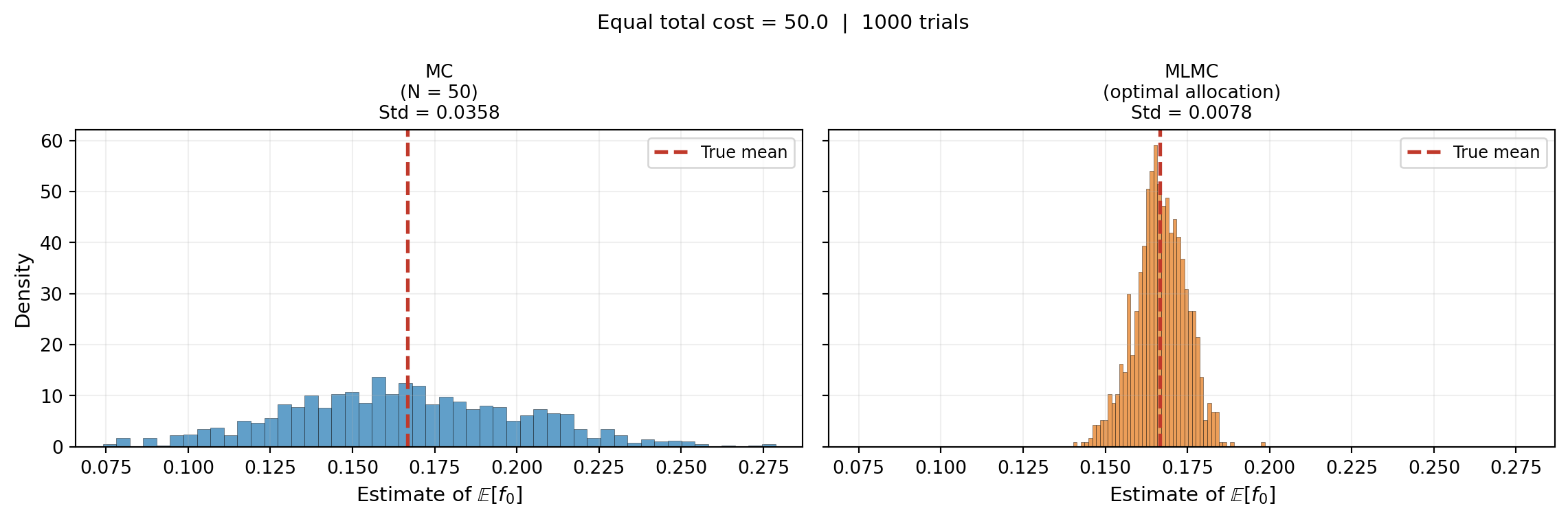
Figure 2 shows histograms of MC and MLMC mean estimates at equal total cost for the five-level polynomial hierarchy. MLMC is dramatically more concentrated around the true mean: the same budget buys far more accuracy by spreading samples intelligently across the hierarchy.
MLMC vs ACV: Same Idea, Different Structure
MLMC is a special case of ACV. To see this, note that for two models the MLMC estimator is
\[ \hat{\mu}_0^{\text{ML}} = \hat{Y}_0 + \hat{Y}_1 = \hat{\mu}_0(\mathcal{Z}_0) - \hat{\mu}_1(\mathcal{Z}_0) + \hat{\mu}_1(\mathcal{Z}_1) = \hat{\mu}_0(\mathcal{Z}_0) - \bigl(\hat{\mu}_1(\mathcal{Z}_0) - \hat{\mu}_1(\mathcal{Z}_1)\bigr) \]
which is exactly the ACV estimator with \(\eta = -1\) fixed. MLMC does not optimise \(\eta\); instead it relies on the hierarchy structure to ensure that \(\eta = -1\) is approximately optimal when consecutive model differences are small. The MLMC Analysis tutorial explores the conditions under which this fixed-\(\eta\) structure is efficient.
When Is MLMC a Good Choice?
MLMC thrives when:
- Models form a natural hierarchy where each level is a systematic refinement of the next (mesh refinement, time-step reduction, polynomial order)
- Consecutive corrections are small: \(\mathbb{V}[Y_\ell]\) decreases rapidly toward cheaper levels
- The cost ratio between adjacent levels is large, so cheap levels can absorb many samples
MLMC is less suited when models are not naturally ordered (unrelated surrogates, black-box codes) or when the variance of level corrections does not decrease fast enough to offset the cost of extra model evaluations.
Key Takeaways
- MLMC decomposes \(\mathbb{E}[f_0]\) via a telescoping sum; each term is a level correction \(\mathbb{E}[f_\ell - f_{\ell+1}]\) estimated on an independent sample set
- The estimator variance splits additively: \(\sum_\ell \mathbb{V}[Y_\ell]/N_\ell\)
- Small correction variances at cheap levels allow large \(N_\ell\) at low cost, driving overall variance down
- MLMC is a special case of ACV with \(\eta = -1\) fixed
Exercises
For the identity Equation 1 to hold, \(f_{M+1}\) must equal zero. What would change if we set \(f_{M+1}\) to a non-zero constant instead?
Suppose \(\mathbb{V}[Y_\ell] = V_0 \cdot 4^{-\ell}\) and \(C_\ell = C_0 \cdot 4^{-\ell}\). Sketch how \(N_\ell\) should grow or shrink with \(\ell\) to keep each term in Equation 3 equal.
MLMC uses independent sample sets across levels. What would go wrong if the same samples were used at every level?
Next Steps
- MLMC Analysis — Derive optimal sample allocation and the MLMC complexity theorem
- API Cookbook — Run MLMC with the PyApprox API
- Multi-Fidelity Monte Carlo — An alternative hierarchy estimator with a different sample-sharing structure
Tip
Ready to try this? See API Cookbook → MLMCEstimator.
References
[GOR2008] M.B. Giles. Multilevel Monte Carlo path simulation. Operations Research, 56(3):607–617, 2008. DOI
[CGSTCVS2011] K.A. Cliffe, M.B. Giles, R. Scheichl, A.L. Teckentrup. Multilevel Monte Carlo methods and applications to elliptic PDEs with random coefficients. Computing and Visualization in Science, 14:3–15, 2011. DOI