---
title: "What Makes a Good Surrogate?"
subtitle: "PyApprox Tutorial Library"
description: "How the choice of ansatz, training data, and fitting strategy affect surrogate quality, and how different surrogates exploit different kinds of function structure."
tutorial_type: conceptual
topic: surrogate_modeling
difficulty: beginner
estimated_time: 12
prerequisites:
- surrogate_workflow
tags:
- surrogate
- polynomial-chaos
- gaussian-process
- function-train
- sparse-grid
- sampling
format:
html:
code-fold: false
code-tools: true
toc: true
execute:
echo: true
warning: false
jupyter: python3
---
::: {.callout-tip collapse="true"}
## Download Notebook
[Download as Jupyter Notebook](notebooks/surrogate_design.ipynb)
:::
## Learning Objectives
After completing this tutorial, you will be able to:
- Explain why the surrogate's basis must match the function's structure
- Describe what kinds of structure different surrogate methods exploit: polynomial
smoothness, anisotropy, low rank, and kernel regularity
- Explain why sample placement affects surrogate quality and how quasi-Monte Carlo
improves on random sampling
- Describe the curse of dimensionality and why structure exploitation is essential in
high dimensions
## The Ansatz Must Match the Function
In [The Surrogate Modeling Workflow](surrogate_workflow.qmd) we saw that the ansatz ---
the functional form of the surrogate --- constrains what it can represent. This is the
single most consequential decision in the workflow. A poor ansatz cannot be rescued by
more data or a better fitting algorithm.
The essential question is: **does the basis contain functions that look like the target?**
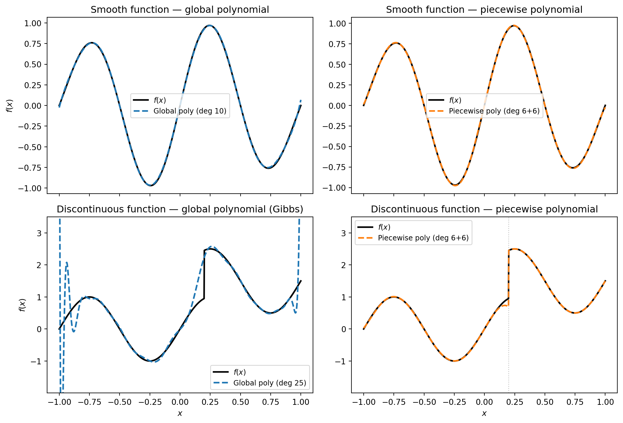
### Smooth Functions: Global Polynomials Work Well
Consider a smooth function like $f(x) = \sin(2\pi x)\,e^{-x^2/2}$. A global polynomial
basis can approximate it to high accuracy because smooth functions have rapidly decaying
polynomial expansion coefficients. As the degree increases, the surrogate converges
quickly.
### Discontinuous Functions: Global Polynomials Fail
Now consider a function with a jump discontinuity. A global polynomial is infinitely
differentiable everywhere --- it is structurally incapable of representing a sharp jump.
No matter how many terms we add, the polynomial will overshoot and oscillate near the
discontinuity. This is the **Gibbs phenomenon**, and it is a fundamental limitation of
smooth bases applied to non-smooth functions.
A **piecewise polynomial** basis, by contrast, can place a breakpoint at (or near) the
discontinuity and represent each smooth piece independently.
```{python}
#| echo: false
#| fig-cap: "Top row: a smooth function approximated by a global polynomial (left) and a piecewise polynomial (right). Both work well, but the global polynomial is more efficient — it needs fewer terms. Bottom row: a discontinuous function. The global polynomial oscillates wildly near the jump (Gibbs phenomenon), while the piecewise polynomial handles it cleanly."
#| label: fig-ansatz-vs-structure
import numpy as np
import matplotlib.pyplot as plt
from pyapprox.util.backends.numpy import NumpyBkd
from pyapprox.probability import UniformMarginal
from pyapprox.surrogates.affine.expansions import create_pce_from_marginals
from pyapprox.surrogates.affine.expansions.fitters import LeastSquaresFitter
_bkd = NumpyBkd()
_marginals = [UniformMarginal(-1.0, 1.0, _bkd)]
x = np.linspace(-1, 1, 1000)
# ── Smooth function ──────────────────────────────────────────────────────────
f_smooth = np.sin(2 * np.pi * x) * np.exp(-x**2 / 2)
# ── Discontinuous function (jump at x = 0.2) ────────────────────────────────
def f_discontinuous(x):
return np.where(x < 0.2,
np.sin(2 * np.pi * x),
np.sin(2 * np.pi * x) + 1.5)
f_disc = f_discontinuous(x)
# ── Fit: global polynomial ───────────────────────────────────────────────────
np.random.seed(10)
N_fit = 60
x_fit = np.random.uniform(-1, 1, N_fit)
_x_eval = _bkd.asarray(x.reshape(1, -1))
_x_fit_2d = _bkd.asarray(x_fit.reshape(1, -1))
_ls = LeastSquaresFitter(_bkd)
# Smooth target
f_fit_smooth = np.sin(2 * np.pi * x_fit) * np.exp(-x_fit**2 / 2)
_pce_smooth = create_pce_from_marginals(_marginals, max_level=10, bkd=_bkd, nqoi=1)
_pce_smooth = _ls.fit(_pce_smooth, _x_fit_2d, _bkd.asarray(f_fit_smooth.reshape(1, -1))).surrogate()
# Discontinuous target
f_fit_disc = f_discontinuous(x_fit)
_pce_disc = create_pce_from_marginals(_marginals, max_level=25, bkd=_bkd, nqoi=1)
_pce_disc = _ls.fit(_pce_disc, _x_fit_2d, _bkd.asarray(f_fit_disc.reshape(1, -1))).surrogate()
# ── Fit: piecewise polynomial ────────────────────────────────────────────────
def fit_piecewise(x_fit, f_fit, x_eval, breakpoint=0.2, deg=5):
"""Fit separate polynomials on each side of a breakpoint."""
mask_left_fit = x_fit < breakpoint
mask_right_fit = x_fit >= breakpoint
mask_left_eval = x_eval < breakpoint
mask_right_eval = x_eval >= breakpoint
result = np.empty_like(x_eval)
if np.sum(mask_left_fit) > deg + 1:
c_left = np.polyfit(x_fit[mask_left_fit], f_fit[mask_left_fit], deg)
result[mask_left_eval] = np.polyval(c_left, x_eval[mask_left_eval])
else:
result[mask_left_eval] = np.nan
if np.sum(mask_right_fit) > deg + 1:
c_right = np.polyfit(x_fit[mask_right_fit], f_fit[mask_right_fit], deg)
result[mask_right_eval] = np.polyval(c_right, x_eval[mask_right_eval])
else:
result[mask_right_eval] = np.nan
return result
pw_smooth = fit_piecewise(x_fit, f_fit_smooth, x, breakpoint=0.0, deg=6)
pw_disc = fit_piecewise(x_fit, f_fit_disc, x, breakpoint=0.2, deg=6)
# ── Four-panel figure ────────────────────────────────────────────────────────
fig, axes = plt.subplots(2, 2, figsize=(11, 7.5), sharex=True)
# Top-left: smooth + global poly
ax = axes[0, 0]
ax.plot(x, f_smooth, "k-", lw=2, label=r"$f(x)$")
ax.plot(x, _bkd.to_numpy(_pce_smooth(_x_eval)).ravel(), "C0--", lw=2, label="Global poly (deg 10)")
ax.set_ylabel(r"$f(x)$")
ax.legend(fontsize=9)
ax.set_title("Smooth function — global polynomial")
# Top-right: smooth + piecewise poly
ax = axes[0, 1]
ax.plot(x, f_smooth, "k-", lw=2, label=r"$f(x)$")
ax.plot(x, pw_smooth, "C1--", lw=2, label="Piecewise poly (deg 6+6)")
ax.legend(fontsize=9)
ax.set_title("Smooth function — piecewise polynomial")
# Bottom-left: discontinuous + global poly
ax = axes[1, 0]
ax.plot(x, f_disc, "k-", lw=2, label=r"$f(x)$")
y_global_disc = _bkd.to_numpy(_pce_disc(_x_eval)).ravel()
ax.plot(x, y_global_disc, "C0--", lw=2, label="Global poly (deg 25)")
ax.set_xlabel(r"$x$")
ax.set_ylabel(r"$f(x)$")
ax.legend(fontsize=9)
ax.set_title("Discontinuous function — global polynomial (Gibbs)")
ax.set_ylim(f_disc.min() - 1.0, f_disc.max() + 1.0)
# Bottom-right: discontinuous + piecewise poly
ax = axes[1, 1]
ax.plot(x, f_disc, "k-", lw=2, label=r"$f(x)$")
ax.plot(x, pw_disc, "C1--", lw=2, label="Piecewise poly (deg 6+6)")
ax.axvline(0.2, color="gray", ls=":", lw=1, alpha=0.5)
ax.set_xlabel(r"$x$")
ax.legend(fontsize=9)
ax.set_title("Discontinuous function — piecewise polynomial")
ax.set_ylim(f_disc.min() - 1.0, f_disc.max() + 1.0)
plt.tight_layout()
plt.show()
```
The lesson is general: every basis encodes assumptions about the target function.
When those assumptions are met, convergence is fast. When they are violated, no amount
of data or optimisation will compensate. The rest of this tutorial surveys how different
surrogate methods encode different structural assumptions.
## Exploiting Structure in Multivariate Functions
In one dimension, choosing between a global and a piecewise polynomial already matters.
In higher dimensions the stakes are much greater, because the **curse of dimensionality**
(discussed below) makes it impossible to approximate a generic $d$-dimensional function
without exploiting some kind of structure.
Different surrogate methods target different structural properties of $f$. Understanding
*what* structure each method exploits is the key to choosing the right tool.
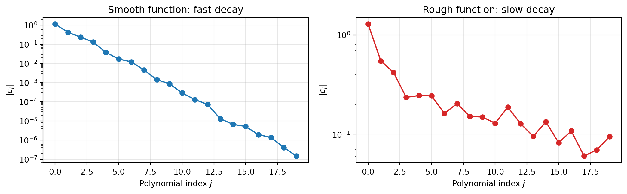
### Polynomial Chaos Expansions: Smoothness and the Input Measure
A **polynomial chaos expansion (PCE)** writes the model output as a sum of multivariate
polynomials:
$$
\hat{f}(\mathbf{x}) = \sum_{j=0}^{P-1} c_j \, \Psi_j(\mathbf{x})
$$
where each $\Psi_j$ is a product of univariate polynomials chosen to be **orthogonal
with respect to the input probability measure**. Gaussian inputs get Hermite
polynomials, uniform inputs get Legendre polynomials, and so on.
The structure that PCE exploits is **smoothness**: if $f$ is smooth, its polynomial
expansion coefficients decay rapidly, so a moderate number of terms gives a good
approximation. The connection to the input measure is a bonus --- orthogonality means
the expansion coefficients directly encode statistical moments, making downstream UQ
essentially free once the surrogate is fitted.
```{python}
#| echo: false
#| fig-cap: "PCE coefficients for a smooth function (left) decay rapidly — a few terms capture most of the variance. For a rough function (right) the coefficients decay slowly, requiring many more terms for the same accuracy."
#| label: fig-pce-coefficient-decay
fig, axes = plt.subplots(1, 2, figsize=(11, 3.5))
# Smooth function: fast coefficient decay
np.random.seed(42)
n_terms = 20
smooth_coeffs = np.exp(-0.8 * np.arange(n_terms)) * (
1 + 0.3 * np.random.randn(n_terms)
)
smooth_coeffs = np.abs(smooth_coeffs)
ax = axes[0]
ax.semilogy(range(n_terms), smooth_coeffs, "C0o-", ms=6, lw=1.5)
ax.set_xlabel("Polynomial index $j$")
ax.set_ylabel(r"$|c_j|$")
ax.set_title("Smooth function: fast decay")
ax.grid(True, alpha=0.3)
# Rough function: slow coefficient decay
rough_coeffs = 1.0 / (1 + np.arange(n_terms))**0.8 * (
1 + 0.2 * np.random.randn(n_terms)
)
rough_coeffs = np.abs(rough_coeffs)
ax = axes[1]
ax.semilogy(range(n_terms), rough_coeffs, "C3o-", ms=6, lw=1.5)
ax.set_xlabel("Polynomial index $j$")
ax.set_ylabel(r"$|c_j|$")
ax.set_title("Rough function: slow decay")
ax.grid(True, alpha=0.3)
plt.tight_layout()
plt.show()
```
PCEs work best when the function is smooth and the number of important input variables is
moderate. For details on building and fitting a PCE, see
[Building a Polynomial Chaos Surrogate](polynomial_chaos_surrogates.qmd).
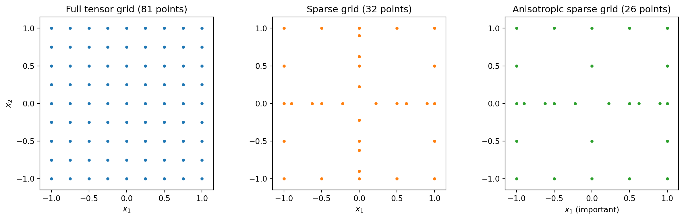
### Sparse Grids: Exploiting Anisotropy
Many multivariate functions are **anisotropic**: some input variables have a much
stronger effect on the output than others. A full tensor-product polynomial basis
allocates the same resolution to every variable, wasting effort on directions that
contribute little.
**Sparse grids** address this by building an approximation from a carefully selected
subset of tensor-product terms. The idea is rooted in the **Smolyak construction**:
instead of requiring high resolution in all $d$ dimensions simultaneously, we combine
many lower-dimensional approximations that each resolve one or two directions well.
```{python}
#| echo: false
#| fig-cap: "Left: a full tensor-product grid in 2D with 9 points per dimension (81 total). Centre: a Smolyak sparse grid at comparable accuracy (32 points). Right: an anisotropic sparse grid that allocates more resolution to the important variable x₁ (26 points). Sparse grids dramatically reduce the number of required evaluations by avoiding the corners of the full grid."
#| label: fig-sparse-grid-points
from itertools import product
fig, axes = plt.subplots(1, 3, figsize=(13, 4))
# Full tensor grid
ax = axes[0]
pts_1d = np.linspace(-1, 1, 9)
xx, yy = np.meshgrid(pts_1d, pts_1d)
ax.plot(xx.ravel(), yy.ravel(), "C0.", ms=6)
ax.set_title(f"Full tensor grid ({len(xx.ravel())} points)")
ax.set_xlabel(r"$x_1$")
ax.set_ylabel(r"$x_2$")
ax.set_xlim(-1.15, 1.15)
ax.set_ylim(-1.15, 1.15)
ax.set_aspect("equal")
# Smolyak sparse grid (level 4, 2D, Clenshaw-Curtis-like)
# Hand-coded representative sparse grid points for illustration
ax = axes[1]
def cc_pts(n):
"""Clenshaw-Curtis points of order n."""
if n == 0:
return np.array([0.0])
return -np.cos(np.pi * np.arange(n + 1) / n)
def smolyak_2d(level):
"""Generate 2D Smolyak sparse grid points (isotropic)."""
points = set()
d = 2
for l1 in range(level + 1):
for l2 in range(level + 1):
if l1 + l2 <= level and l1 + l2 >= max(0, level - d + 1):
p1 = cc_pts(2**l1 - 1 if l1 > 0 else 0)
p2 = cc_pts(2**l2 - 1 if l2 > 0 else 0)
for a, b in product(p1, p2):
points.add((round(a, 10), round(b, 10)))
return np.array(list(points))
sg_pts = smolyak_2d(3)
ax.plot(sg_pts[:, 0], sg_pts[:, 1], "C1.", ms=6)
ax.set_title(f"Sparse grid ({len(sg_pts)} points)")
ax.set_xlabel(r"$x_1$")
ax.set_xlim(-1.15, 1.15)
ax.set_ylim(-1.15, 1.15)
ax.set_aspect("equal")
# Anisotropic sparse grid: more resolution in x1
ax = axes[2]
def smolyak_2d_aniso(level, max_l1, max_l2):
"""Anisotropic Smolyak grid with per-dimension level caps."""
points = set()
d = 2
for l1 in range(min(level, max_l1) + 1):
for l2 in range(min(level, max_l2) + 1):
if l1 + l2 <= level and l1 + l2 >= max(0, level - d + 1):
p1 = cc_pts(2**l1 - 1 if l1 > 0 else 0)
p2 = cc_pts(2**l2 - 1 if l2 > 0 else 0)
for a, b in product(p1, p2):
points.add((round(a, 10), round(b, 10)))
return np.array(list(points))
sg_aniso = smolyak_2d_aniso(3, max_l1=3, max_l2=2)
ax.plot(sg_aniso[:, 0], sg_aniso[:, 1], "C2.", ms=6)
ax.set_title(f"Anisotropic sparse grid ({len(sg_aniso)} points)")
ax.set_xlabel(r"$x_1$ (important)")
ax.set_xlim(-1.15, 1.15)
ax.set_ylim(-1.15, 1.15)
ax.set_aspect("equal")
plt.tight_layout()
plt.show()
```
The key insight is that sparse grids **allocate resolution where it matters**. If $x_1$
drives most of the output variability and $x_2$ has only a mild effect, an anisotropic
sparse grid puts many more points along $x_1$ and only a coarse resolution along $x_2$.
This can reduce the required number of evaluations from $n^d$ (full grid) to something
closer to $n \log(n)^{d-1}$ for isotropic sparse grids, with further savings when
anisotropy is exploited.
### Function Trains: Exploiting Low-Rank Structure
Some multivariate functions have limited **interaction** between their input variables.
A function is **rank-1** (separable) if it can be written as a product of univariate
functions:
$$
f(x_1, x_2) = g_1(x_1) \cdot g_2(x_2)
$$
A **rank-$r$** function is a sum of $r$ such products. Many functions arising in
engineering have low effective rank --- the variables interact, but in a limited way
that can be captured by a modest number of product terms.
The **function train (FT)** decomposition represents a $d$-dimensional function as
a chain of matrix multiplications:
$$
f(x_1, \ldots, x_d) = \mathbf{G}_1(x_1) \cdot \mathbf{G}_2(x_2) \cdots \mathbf{G}_d(x_d)
$$
where each **core** $\mathbf{G}_k(x_k)$ is a matrix whose entries are univariate
functions. The shared matrix dimensions --- the **ranks** --- control how much
interaction between variables the FT can represent.
```{python}
#| echo: false
#| fig-cap: "A rank-1 function (left) is a product of two 1D functions — its contours are perfectly aligned with the coordinate axes. A rank-2 function (centre) is a sum of two such products, enabling richer structure like multiple peaks. A generic function (right) may require many terms, but low-rank approximations often capture most of the variability with surprisingly small rank."
#| label: fig-low-rank
x1 = np.linspace(-1, 1, 200)
x2 = np.linspace(-1, 1, 200)
X1, X2 = np.meshgrid(x1, x2)
# Rank 1: product of Gaussians
Z_rank1 = np.exp(-4 * X1**2) * np.exp(-4 * X2**2)
# Rank 2: sum of two rank-1 terms
Z_rank2 = (np.exp(-8 * (X1 + 0.5)**2) * np.exp(-8 * (X2 + 0.5)**2) +
np.exp(-3 * (X1 - 0.5)**2) * np.exp(-3 * (X2 - 0.5)**2))
# Higher rank / generic
Z_generic = (np.sin(2 * np.pi * X1) * np.cos(np.pi * X2) +
0.5 * np.exp(-3 * ((X1 - 0.3)**2 + (X2 + 0.4)**2)) +
0.3 * X1 * X2**2)
fig, axes = plt.subplots(1, 3, figsize=(13, 4))
for ax, Z, title in zip(
axes,
[Z_rank1, Z_rank2, Z_generic],
["Rank-1 (separable)", "Rank-2 (sum of products)", "Higher rank"],
):
cf = ax.contourf(X1, X2, Z, levels=20, cmap="cividis")
ax.set_xlabel(r"$x_1$")
ax.set_ylabel(r"$x_2$")
ax.set_title(title)
ax.set_aspect("equal")
plt.tight_layout()
plt.show()
```
The computational advantage is dramatic: a full polynomial expansion in $d$ variables at
degree $p$ has $\binom{d+p}{d}$ terms, growing exponentially in $d$. A rank-$r$ function
train has $\mathcal{O}(d \cdot r^2 \cdot p)$ parameters --- **linear in $d$** for fixed
rank. This makes FTs one of the few surrogate methods that scale to truly high-dimensional
problems, provided the function has low effective rank.
For a detailed construction of function trains, see
[An Introduction to Function Trains](function_train_surrogates.qmd).
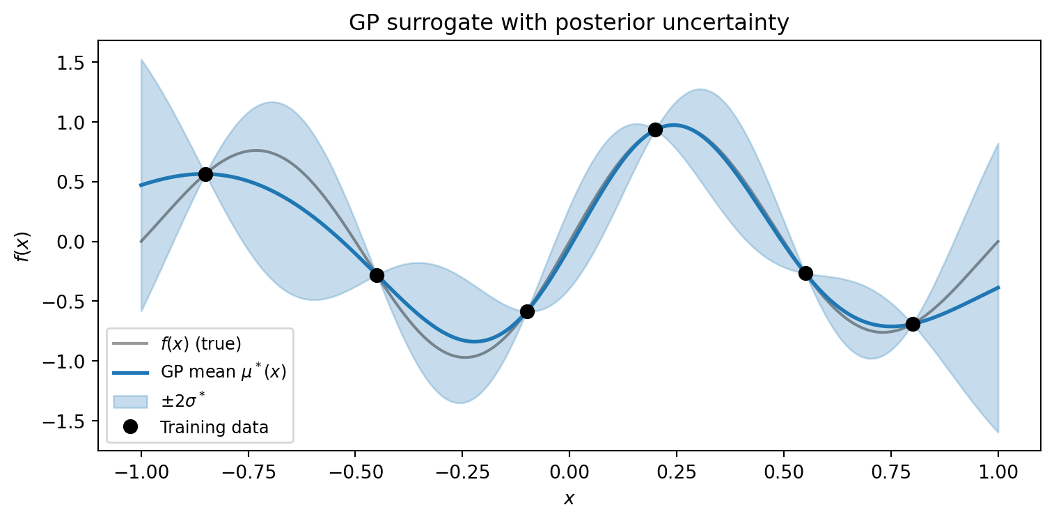
### Gaussian Processes: Kernel-Encoded Smoothness and Uncertainty
A **Gaussian process (GP)** is a probability distribution over functions, defined by a
mean function and a **kernel** $k(\mathbf{x}, \mathbf{x}')$ that encodes assumptions
about the function's smoothness and correlation structure.
The structure a GP exploits is entirely determined by its kernel:
- A **Squared Exponential** kernel assumes the function is infinitely smooth
- A **Matérn 5/2** kernel assumes twice-differentiable functions
- A **Matérn 3/2** kernel allows once-differentiable functions with small-scale roughness
- **Anisotropic length scales** (one per input dimension) let the GP learn which
variables the function varies along most rapidly
The defining advantage of a GP over other surrogates is that it provides built-in
**uncertainty quantification**. At every prediction point, the GP returns not just a
best estimate $\mu^*(\mathbf{x})$ but also a posterior standard deviation
$\sigma^*(\mathbf{x})$ that reflects how far the point is from the training data.
```{python}
#| echo: false
#| fig-cap: "A GP surrogate (blue line) with posterior uncertainty (shaded ±2σ band). Near training points (black dots) the band narrows to near zero — the GP is confident. Between observations the band widens, honestly reporting where the surrogate is uncertain. This built-in uncertainty is the GP's defining feature."
#| label: fig-gp-uncertainty
np.random.seed(7)
# Simple 1D GP illustration
x_grid = np.linspace(-1, 1, 300)
x_obs = np.array([-0.85, -0.45, -0.1, 0.2, 0.55, 0.8])
f_obs = np.sin(2 * np.pi * x_obs) * np.exp(-x_obs**2 / 2)
# Build kernel matrix (SE kernel)
def se_kernel(x1, x2, ell=0.25, sigma=1.0):
return sigma**2 * np.exp(-0.5 * (x1[:, None] - x2[None, :])**2 / ell**2)
K_oo = se_kernel(x_obs, x_obs) + 1e-8 * np.eye(len(x_obs))
K_so = se_kernel(x_grid, x_obs)
K_ss = se_kernel(x_grid, x_grid)
L = np.linalg.cholesky(K_oo)
alpha = np.linalg.solve(L.T, np.linalg.solve(L, f_obs))
mu = K_so @ alpha
v = np.linalg.solve(L, K_so.T)
var = np.diag(K_ss) - np.sum(v**2, axis=0)
std = np.sqrt(np.clip(var, 0, None))
f_grid = np.sin(2 * np.pi * x_grid) * np.exp(-x_grid**2 / 2)
fig, ax = plt.subplots(figsize=(8, 4))
ax.plot(x_grid, f_grid, "k-", lw=1.5, alpha=0.4, label=r"$f(x)$ (true)")
ax.plot(x_grid, mu, "C0-", lw=2, label=r"GP mean $\mu^*(x)$")
ax.fill_between(x_grid, mu - 2*std, mu + 2*std, alpha=0.25, color="C0",
label=r"$\pm 2\sigma^*$")
ax.plot(x_obs, f_obs, "ko", ms=7, zorder=5, label="Training data")
ax.set_xlabel(r"$x$")
ax.set_ylabel(r"$f(x)$")
ax.legend(fontsize=9, loc="lower left")
ax.set_title("GP surrogate with posterior uncertainty")
plt.tight_layout()
plt.show()
```
This uncertainty information is valuable beyond accuracy assessment. It enables
**adaptive sampling** strategies that place new training points where the GP is most
uncertain, systematically filling gaps in data coverage. For details, see
[Building a Gaussian Process Surrogate](gp_surrogate.qmd).
### Neural Networks: Compositional Structure
**Neural network** surrogates learn a hierarchy of nonlinear transformations:
$$
\hat{f}(\mathbf{x}) = W_L \circ \sigma \circ W_{L-1} \circ \cdots \circ \sigma \circ W_1(\mathbf{x})
$$
where $W_\ell$ are affine maps and $\sigma$ is a nonlinear activation. The structure
they exploit is **compositional**: many physical phenomena can be described as a sequence
of simpler transformations applied one after another. Neural networks learn these
intermediate representations from data.
Their flexibility is both a strength and a weakness. Neural networks impose fewer
structural assumptions than polynomials or GPs, making them applicable to a broad class
of functions. But this flexibility means they typically require more training data and
provide no built-in uncertainty quantification. They also lack the direct connection to
the input probability measure that makes PCE-based UQ analytically tractable.
Neural network surrogates are most compelling when the input dimension is very large,
the data is abundant, or the function has compositional structure that other methods
cannot exploit.
### Summary: Which Structure Does Each Method Exploit?
| Method | Structure exploited | Strengths | Limitations |
|---|---|---|---|
| **PCE** | Smoothness, input measure | Analytical UQ, spectral convergence | Curse of dimensionality, assumes smoothness |
| **Sparse grids** | Anisotropy, variable importance | Efficient for anisotropic functions | Still polynomial-based, moderate $d$ |
| **Function trains** | Low-rank variable interactions | Linear scaling in $d$ | Requires low effective rank |
| **GPs** | Kernel smoothness | Built-in uncertainty, adaptive sampling | $\mathcal{O}(N^3)$ fitting cost |
| **Neural networks** | Compositional hierarchy | Flexible, handles large $d$ | Data-hungry, no analytical UQ |
No single method dominates. The right choice depends on the function's structure, the
input dimension, the computational budget, and the downstream task.
## Training Data Design Matters
The second decision in the surrogate workflow is **where to sample**. Even with the
right ansatz, poor sample placement can produce a poor surrogate.
### Random Sampling Leaves Gaps
Random Monte Carlo sampling is simple: draw $N$ points independently from the input
distribution. But random points tend to cluster in some regions and leave gaps in
others. In 2D the effect is visible; in higher dimensions it becomes severe.
### Quasi-Monte Carlo: Better Coverage
**Quasi-Monte Carlo (QMC)** sequences --- such as Sobol, Halton, or lattice rules --- are
deterministic point sets designed to fill the domain more evenly than random samples.
They minimise the **discrepancy** (a measure of how unevenly the points cover the
space).
```{python}
#| echo: false
#| fig-cap: "256 sample points in 2D drawn by Monte Carlo (left) and a Sobol quasi-Monte Carlo sequence (right). The MC samples cluster and leave visible gaps. The Sobol sequence covers the domain much more uniformly, which translates directly to better surrogate accuracy for the same number of evaluations."
#| label: fig-mc-vs-qmc
from pyapprox.util.backends.numpy import NumpyBkd as _NumpyBkd
from pyapprox.expdesign.quadrature import SobolSampler
_bkd = _NumpyBkd()
np.random.seed(17)
N_pts = 256
fig, axes = plt.subplots(1, 2, figsize=(10, 4.5))
# Monte Carlo
ax = axes[0]
mc_pts = np.random.uniform(0, 1, (N_pts, 2))
ax.plot(mc_pts[:, 0], mc_pts[:, 1], "C0.", ms=4, alpha=0.7)
ax.set_title(f"Monte Carlo ($N = {N_pts}$)")
ax.set_xlabel(r"$x_1$")
ax.set_ylabel(r"$x_2$")
ax.set_xlim(-0.02, 1.02)
ax.set_ylim(-0.02, 1.02)
ax.set_aspect("equal")
# Sobol QMC via PyApprox
ax = axes[1]
_sobol = SobolSampler(2, _bkd, scramble=True, seed=42)
qmc_pts, _ = _sobol.sample(N_pts)
qmc_pts_np = _bkd.to_numpy(qmc_pts)
ax.plot(qmc_pts_np[0], qmc_pts_np[1], "C1.", ms=4, alpha=0.7)
ax.set_title(f"Sobol QMC ($N = {N_pts}$)")
ax.set_xlabel(r"$x_1$")
ax.set_xlim(-0.02, 1.02)
ax.set_ylim(-0.02, 1.02)
ax.set_aspect("equal")
plt.tight_layout()
plt.show()
```
### Better Coverage → Better Surrogates
The improved space-filling of QMC translates directly to better surrogate accuracy for the
same $N$. The following experiment fits the same polynomial surrogate to 1D training data
drawn by MC and QMC, repeated over many random seeds to show the variability.
```{python}
#| echo: false
#| fig-cap: "Surrogate error vs. number of training points for Monte Carlo (blue) and Sobol QMC (orange) sampling. Bands show the 10th–90th percentile range over 50 repetitions (QMC uses different scrambles). QMC consistently achieves lower error with less variability, especially at small N where every sample point matters most."
#| label: fig-sampling-convergence
def f_1d(x):
return np.sin(3 * np.pi * x) * np.exp(-x**2)
x_test_1d = np.linspace(-1, 1, 1000)
f_test_1d = f_1d(x_test_1d)
oversample = 2
degrees_conv = list(range(2, 26))
N_values = [oversample * (p + 1) for p in degrees_conv]
n_reps = 50
_x_test_2d = _bkd.asarray(x_test_1d.reshape(1, -1))
mc_errors = np.zeros((len(degrees_conv), n_reps))
qmc_errors = np.zeros((len(degrees_conv), n_reps))
for i, (p, N) in enumerate(zip(degrees_conv, N_values)):
for rep in range(n_reps):
# MC
rng = np.random.default_rng(rep * 1000 + i)
x_mc = rng.uniform(-1, 1, N)
_s_mc = _bkd.asarray(x_mc.reshape(1, -1))
_v_mc = _bkd.asarray(f_1d(x_mc).reshape(1, -1))
_pce_mc = create_pce_from_marginals(_marginals, max_level=p, bkd=_bkd, nqoi=1)
_pce_mc = LeastSquaresFitter(_bkd).fit(_pce_mc, _s_mc, _v_mc).surrogate()
_fhat_mc = _bkd.to_numpy(_pce_mc(_x_test_2d)).ravel()
mc_errors[i, rep] = (np.linalg.norm(f_test_1d - _fhat_mc)
/ np.linalg.norm(f_test_1d))
# QMC (Sobol, scrambled) via PyApprox
_sobol_1d = SobolSampler(1, _bkd, scramble=True, seed=rep * 1000 + i)
x_qmc_arr, _ = _sobol_1d.sample(N)
x_qmc = _bkd.to_numpy(x_qmc_arr).ravel() * 2 - 1 # map [0,1] -> [-1,1]
_s_qmc = _bkd.asarray(x_qmc.reshape(1, -1))
_v_qmc = _bkd.asarray(f_1d(x_qmc).reshape(1, -1))
_pce_qmc = create_pce_from_marginals(_marginals, max_level=p, bkd=_bkd, nqoi=1)
_pce_qmc = LeastSquaresFitter(_bkd).fit(_pce_qmc, _s_qmc, _v_qmc).surrogate()
_fhat_qmc = _bkd.to_numpy(_pce_qmc(_x_test_2d)).ravel()
qmc_errors[i, rep] = (np.linalg.norm(f_test_1d - _fhat_qmc)
/ np.linalg.norm(f_test_1d))
fig, ax = plt.subplots(figsize=(7, 4.5))
mc_med = np.median(mc_errors, axis=1)
mc_lo = np.percentile(mc_errors, 10, axis=1)
mc_hi = np.percentile(mc_errors, 90, axis=1)
qmc_med = np.median(qmc_errors, axis=1)
qmc_lo = np.percentile(qmc_errors, 10, axis=1)
qmc_hi = np.percentile(qmc_errors, 90, axis=1)
ax.loglog(N_values, mc_med, "C0o-", lw=2, ms=6, label="MC (median)")
ax.fill_between(N_values, mc_lo, mc_hi, alpha=0.15, color="C0")
ax.loglog(N_values, qmc_med, "C1s-", lw=2, ms=6, label="QMC Sobol (median)")
ax.fill_between(N_values, qmc_lo, qmc_hi, alpha=0.15, color="C1")
ax.set_xlabel("Training points $N$")
ax.set_ylabel(r"Relative $L_2$ error")
ax.set_title("Sample design affects surrogate accuracy")
ax.legend()
ax.grid(True, alpha=0.3)
plt.tight_layout()
plt.show()
```
The practical message: **before spending the budget on more evaluations, consider
whether the same budget spent on better-placed evaluations would help more.** This
is especially important when each evaluation is expensive and the budget is small.
## The Curse of Dimensionality
Everything above becomes dramatically harder in high dimensions. To understand why,
consider the simplest approach to approximating a $d$-dimensional function: evaluate
it on a grid.
With $n$ points per dimension, the total number of grid points is $n^d$. Even a modest
$n = 10$ becomes completely infeasible in moderate dimensions:
```{python}
#| echo: false
#| fig-cap: "The curse of dimensionality: grid points required for n = 10 points per dimension. At d = 5 we already need 100,000 evaluations. By d = 10, the count exceeds any computational budget. This exponential scaling is why surrogate methods must exploit function structure — smoothness, anisotropy, low rank — to break the curse."
#| label: fig-curse-of-dimensionality
fig, axes = plt.subplots(1, 2, figsize=(12, 4))
# Left: grid points in 1D, 2D, 3D
ax = axes[0]
np.random.seed(0)
# 1D
pts_1d = np.linspace(0, 1, 5)
y_1d = 2.2
ax.plot(pts_1d, [y_1d]*len(pts_1d), "C0o", ms=8)
ax.text(0.5, y_1d + 0.1, f"1D: {len(pts_1d)} points", ha="center", fontsize=10)
# 2D
pts_2d_x, pts_2d_y = np.meshgrid(np.linspace(0, 1, 5), np.linspace(0, 1, 5))
offset_y = 0.0
ax.plot(pts_2d_x.ravel(), pts_2d_y.ravel() + offset_y, "C1o", ms=4)
ax.text(0.5, 1.2, f"2D: {pts_2d_x.size} points", ha="center", fontsize=10)
ax.set_xlim(-0.1, 1.1)
ax.set_ylim(-0.3, 2.6)
ax.set_aspect("equal")
ax.axis("off")
ax.set_title("Grid points: $n = 5$", fontsize=11)
# Right: exponential growth
ax = axes[1]
dims = np.arange(1, 16)
n_per_dim = 10
grid_sizes = n_per_dim ** dims
ax.semilogy(dims, grid_sizes, "C3o-", ms=7, lw=2)
ax.axhline(1e6, color="gray", ls="--", lw=1, alpha=0.6)
ax.text(12, 1.5e6, "$10^6$ (practical limit)", fontsize=9, color="gray")
ax.set_xlabel("Number of dimensions $d$")
ax.set_ylabel("Grid points ($n^d$)")
ax.set_title("Exponential growth: $n = 10$", fontsize=11)
ax.grid(True, alpha=0.3)
ax.set_xticks(range(1, 16, 2))
plt.tight_layout()
plt.show()
```
This is why **exploiting structure is not optional in high dimensions --- it is the
only way forward**:
- **PCEs** with total-degree index sets grow as $\binom{d+p}{d}$ instead of $p^d$, but
this is still exponential for fixed $p$. Sparse and low-rank PCE methods push this
further.
- **Sparse grids** reduce the grid count to $\mathcal{O}(n \log(n)^{d-1})$, exploiting
the fact that most grid points in a full tensor product contribute negligibly.
- **Function trains** scale as $\mathcal{O}(d \cdot r^2 \cdot p)$ --- linear in $d$ ---
by exploiting low-rank interaction structure.
- **GPs** bypass the grid entirely by placing a continuous prior over functions, but
their fitting cost $\mathcal{O}(N^3)$ limits them to moderate training set sizes.
The right surrogate method is the one that **matches the structure your function
actually has**, allowing it to break the exponential scaling barrier.
## Key Takeaways
- The **ansatz must match the function's structure**. Global polynomials excel for smooth
functions but fail for discontinuities; piecewise bases handle jumps but are less
efficient for smooth targets. This mismatch is the most common source of poor
surrogate performance.
- Different surrogate methods exploit different structures: **PCE** exploits smoothness
and the input measure, **sparse grids** exploit anisotropy, **function trains** exploit
low-rank interactions, **GPs** encode smoothness via kernels and provide uncertainty,
and **neural networks** exploit compositional hierarchy.
- **Sample placement** affects surrogate quality as much as sample count. Quasi-Monte
Carlo sequences provide better coverage than random sampling for the same budget.
- The **curse of dimensionality** makes structure exploitation essential, not optional,
in high dimensions. The surrogate method should be chosen based on what structural
properties the target function is expected to have.
## Next Steps
- [Building a Polynomial Chaos Surrogate](polynomial_chaos_surrogates.qmd) --- Fit a PCE
to an engineering benchmark and assess accuracy
- [Building a Gaussian Process Surrogate](gp_surrogate.qmd) --- Fit a GP with
uncertainty quantification and adaptive sampling
- [An Introduction to Function Trains](function_train_surrogates.qmd) --- Build
intuition for low-rank decompositions and the FT representation