
General Approximate Control Variates
PyApprox Tutorial Library
How using all low-fidelity models as direct control variates for the high-fidelity model breaks the CV-1 variance ceiling that limits MLMC and MFMC.
TipDownload Notebook
Learning Objectives
After completing this tutorial, you will be able to:
- Explain why MLMC and MFMC both plateau at the one-model CV-1 variance ceiling
- Contrast indirect correction (MLMC/MFMC recursive chain) with direct correction (every LF model corrects \(f_0\) simultaneously)
- Predict which variance ceiling is reachable for a given model hierarchy
- Identify the settings in which switching from MFMC to a general ACV estimator pays off
Prerequisites
Complete Multi-Fidelity Monte Carlo before this tutorial.
The Ceiling That MFMC Cannot Break
The MFMC Concept tutorial showed that both MFMC and MLMC plateau at a hard variance floor as LF samples grow:
\[ \min\,\mathbb{V}[\hat{\mu}_0^{\text{MFMC}}] \;\xrightarrow{r\to\infty}\; \frac{\sigma_0^2}{N_0}(1 - \rho_{0,1}^2). \]
This is the CV-1 ceiling — the variance reduction achievable if the mean of the single most informative LF model were known exactly. Adding more LF samples or more LF models beyond \(f_1\) does not lower this floor: it only makes the estimator converge to it faster.
The reason is structural. In both MLMC and MFMC, models \(f_\alpha\) for \(\alpha \geq 2\) act as control variates for \(f_{\alpha-1}\), not for \(f_0\). They improve the correction provided by \(f_1\), but each model in the chain can only reduce variance in the step above it. Only \(f_1\) is wired directly into the HF estimator \(\hat{\mu}_0(\mathcal{Z}_0)\). This is the indirect correction structure.
What if instead every LF model’s correction were applied directly to \(\hat{\mu}_0\)?
Direct vs Indirect Correction
The structural difference is visible before any algebra.
MFMC / MLMC (indirect): The correction chain runs \(f_M \to f_{M-1} \to \cdots \to f_1 \to f_0\). Each model sharpens the correction provided by the model above it in the hierarchy. Only \(f_1\) directly reduces the variance of \(\hat{\mu}_0(\mathcal{Z}_0)\).
General ACV — direct correction: Every LF model simultaneously corrects \(f_0\). The estimator is
\[ \hat{\mu}_0^{\text{ACV}} = \hat{\mu}_0(\mathcal{Z}_0) + \sum_{\alpha=1}^{M} \eta_\alpha \bigl(\hat{\mu}_\alpha(\mathcal{Z}_\alpha^*) - \hat{\mu}_\alpha(\mathcal{Z}_\alpha)\bigr), \tag{1}\]
where \(\hat{\mu}_\alpha(\mathcal{Z}_\alpha^*) - \hat{\mu}_\alpha(\mathcal{Z}_\alpha)\) is the correction term for model \(\alpha\): it is unbiased for zero, so the estimator remains unbiased for any weights \(\eta_\alpha\).
This looks identical to the MFMC estimator — and algebraically it is. What differs is the sample-set structure. In MFMC, \(\mathcal{Z}_\alpha^* = \mathcal{Z}_{\alpha-1}\) (each model anchors on the model above it in the chain). In the ACVMF estimator, \(\mathcal{Z}_\alpha^* = \mathcal{Z}_0\) for every \(\alpha\): all LF models share the HF sample set as their comparison point. Each correction is therefore directly correlated with \(\hat{\mu}_0(\mathcal{Z}_0)\), and each one can reduce HF variance independently.
Figure 1 makes this structural difference visual.
Breaking the Ceiling
When all LF models correct \(f_0\) directly and have access to enough exclusive samples, the variance of the ACVMF estimator converges to the multi-model CV limit — the reduction achievable if all LF means were known exactly simultaneously. This limit depends on the joint correlation between \(f_0\) and all LF models, not just the pairwise correlation with \(f_1\).
Figure 2 shows this on the five-model polynomial benchmark.
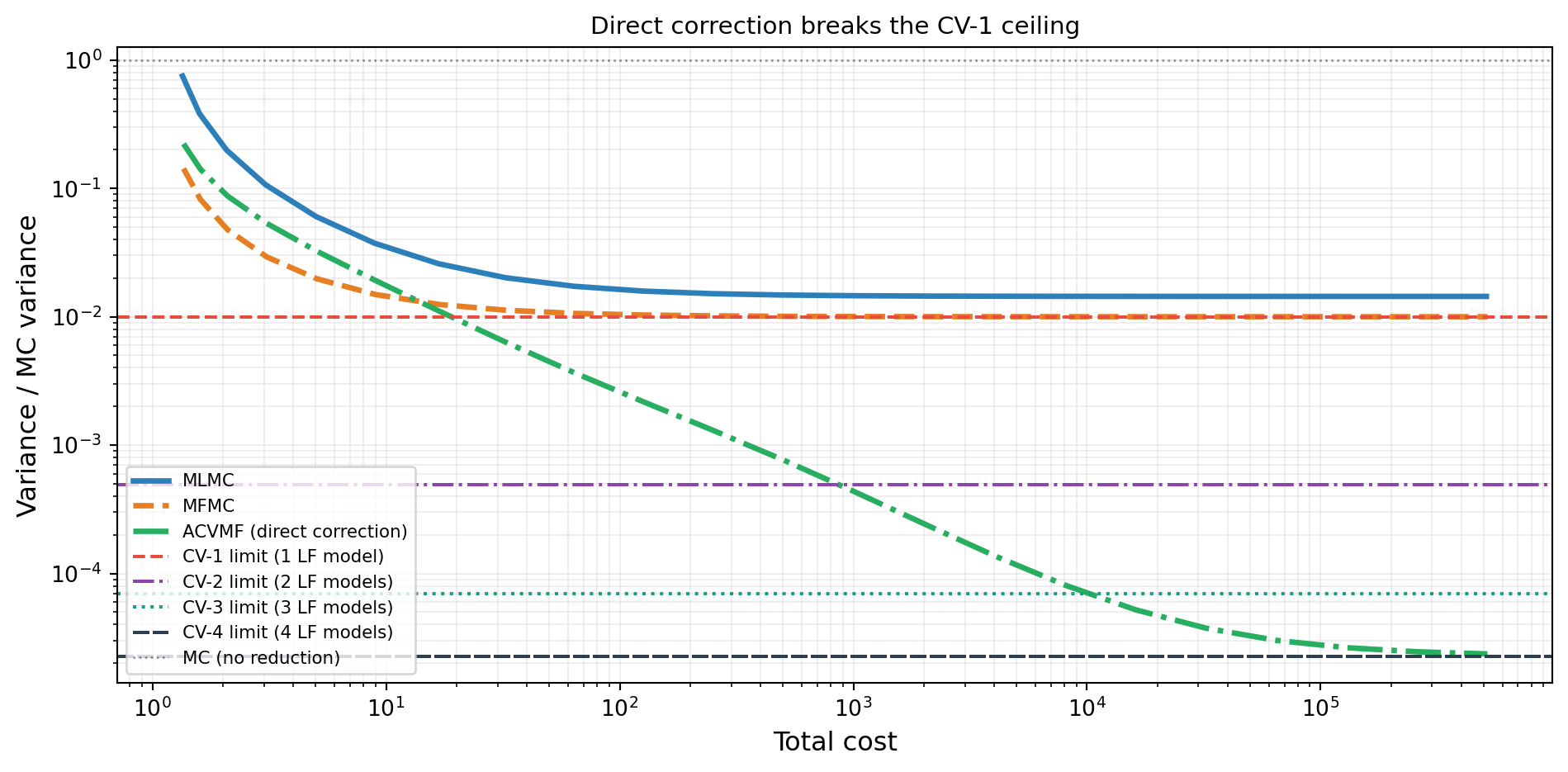
The green curve converges to the CV-4 limit — the reduction possible when all four LF models simultaneously correct \(f_0\). MFMC and MLMC are bounded by the much higher CV-1 limit regardless of how many additional LF samples are added.
Why? Because in Equation 1 with \(\mathcal{Z}_\alpha^* = \mathcal{Z}_0\) for every \(\alpha\), the optimal weights exploit the full joint covariance between \(\hat{\mu}_0(\mathcal{Z}_0)\) and all \(M\) corrections simultaneously. The resulting variance reduction — shown in General ACV Analysis to be a multi-model Schur complement — is at least as large as using any single correction alone, and often much larger.
Note, however, that Figure 2 also shows MFMC outperforming ACVMF at small total costs. Moreover, the plot above holds the HF sample count fixed at \(N_0 = 1\). When the optimizer is free to jointly choose \(N_0\) and the LF partition sizes, MFMC can outperform ACVMF on problems whose models form a natural hierarchy ordered by correlation per unit cost — for example, models obtained by successive mesh refinement. In such hierarchies the chained correction structure of MFMC aligns with the cost–accuracy ordering, and the indirect path through \(f_1\) is already highly efficient. The general ACV framework pays off most when the LF models do not form a hierarchy but are still correlated with the HF model.
The Allocation Problem
As with the two-model ACV estimator, the goal is to minimize estimator variance subject to a computational budget. The estimator’s sample design is built from \(M+1\) independent partitions \(\mathcal{P}_0, \mathcal{P}_1, \ldots, \mathcal{P}_M\) with sample counts \(m_0, m_1, \ldots, m_M\). Which models are evaluated on which partitions is determined by the allocation matrix — the structural choice that distinguishes MLMC, MFMC, and ACVMF. For ACVMF with four models, the allocation matrix assigns:
- \(\mathcal{P}_0\) (\(m_0\) samples): all models \(\{f_0, f_1, f_2, f_3\}\) — the shared HF partition
- \(\mathcal{P}_1\) (\(m_1\) samples): models \(\{f_1, f_2, f_3\}\) — LF only
- \(\mathcal{P}_2\) (\(m_2\) samples): models \(\{f_2, f_3\}\)
- \(\mathcal{P}_3\) (\(m_3\) samples): model \(\{f_3\}\) only
The total number of samples for model \(\alpha\) is the sum across all partitions it appears in. For ACVMF: \(N_0 = m_0\), \(N_1 = m_0 + m_1\), \(N_2 = m_0 + m_1 + m_2\), and so on — the cheapest model accumulates the most samples.
The total cost is \[ P = \sum_{k=0}^{M} m_k\, c^k, \] where \(c^k = \sum_{\alpha \in \mathcal{P}_k} c_\alpha\) is the per-sample cost of partition \(k\).
Writing \(r_k = m_k / m_0\) for the partition ratios (with \(r_0 = 1\)), the budget determines \(m_0\): \[ m_0 = \frac{P}{c^0 + \sum_{k=1}^{M} r_k\, c^k}. \]
The weights \(\boldsymbol{\eta}\) are optimal in closed form for any fixed allocation (see General ACV Analysis). After plugging in \(\boldsymbol{\eta}^*\), the allocation problem reduces to
\[ \min_{r_1, \ldots, r_M \geq 0} \; \mathbb{V}\!\left[\hat{\mu}_0^{\text{ACV}}\right]_{\boldsymbol{\eta}=\boldsymbol{\eta}^*} \quad \text{subject to} \quad m_0\!\left(c^0 + \sum_{k=1}^{M} r_k\, c^k\right) \leq P, \tag{2}\]
an \(M\)-dimensional optimization over the partition ratios. Unlike the two-model case — where the single ratio \(r\) has a closed-form optimum — the many-model allocation requires numerical optimization. PyApprox uses a chained optimizer (differential evolution for global exploration followed by trust-constr for local refinement) by default; see the API Cookbook for configuration details.
The key trade-off is the same as in the two-model case, replicated across partitions: enlarging any partition tightens the corrections it supports but leaves fewer resources for \(m_0\), which controls the baseline HF variance \(\sigma_0^2 / m_0\). The optimizer balances these competing effects jointly.
Key Takeaways
- Both MLMC and MFMC plateau at the one-model CV-1 ceiling; only \(f_1\) directly reduces \(\hat{\mu}_0\) variance in either estimator
- The ceiling is structural — a consequence of the recursive correction chain, not suboptimal weights
- General ACV estimators (e.g. ACVMF) route every LF model’s correction directly to \(\hat{\mu}_0\), approaching the multi-model CV-\(M\) ceiling
- The payoff is largest when several moderately correlated LF models exist and the gap between CV-1 and CV-\(M\) is large
- The gap can be estimated from the pilot covariance alone using the
cv_limitfunction above before committing to any sample budget
Exercises
From Figure 2, at approximately what LF-to-HF ratio does ACVMF achieve half the variance of MFMC at the same ratio?
Suppose \(\rho_{0,1} = 0.95\) and \(\rho_{0,\alpha} = 0.6\) for all \(\alpha \geq 2\). Compute the CV-1 and CV-\(M\) limits as \(M\) grows from 1 to 5. At what \(M\) does the incremental gain become less than 1% of MC variance?
Explain in one sentence why fixing \(\mathcal{Z}_\alpha^* = \mathcal{Z}_0\) for every \(\alpha\) in Equation 1 is the structural change that breaks the CV-1 ceiling.
Next Steps
- General ACV Analysis — Derive the optimal weight matrix \(\mathbf{H}^*\), the minimum covariance formula, and visualise allocation matrices for MLMC, MFMC, ACVMF, and ACVIS
Tip
Ready to try this? See API Cookbook → ACVSearch.
References
[GGEJJCP2020] A. Gorodetsky, S. Geraci, M. Eldred, J. Jakeman. A generalized approximate control variate framework for multifidelity uncertainty quantification. Journal of Computational Physics, 408:109257, 2020. DOI
[PWGSIAM2016] B. Peherstorfer, K. Willcox, M. Gunzburger. Optimal model management for multifidelity Monte Carlo estimation. SIAM Journal on Scientific Computing, 38(5):A3163–A3194, 2016. DOI