Model Ensemble Selection
PyApprox Tutorial Library
Why adding a poorly-correlated low-fidelity model can increase estimator variance relative to using fewer models, and how to automatically identify the best model subset from pilot data alone.
TipDownload Notebook
Learning Objectives
After completing this tutorial, you will be able to:
- Explain why including a weakly-correlated low-fidelity model can increase estimator variance compared to using a smaller ensemble
- Describe the ensemble selection problem: finding the subset \(\mathcal{M}^* \subseteq \{0,\ldots,M\}\) that minimises predicted variance at a given budget
- Interpret a model correlation heatmap to visually identify candidate LF models
- Sketch the enumeration strategy that PyApprox uses to solve the selection problem
Prerequisites
Complete PACV Concept or MLBLUE Concept before this tutorial. Ensemble selection is the final degree of freedom in the multi-fidelity design problem: once the estimator family and sample allocation strategy are chosen, you still need to decide which models to include.
The Surprising Cost of Useless Models
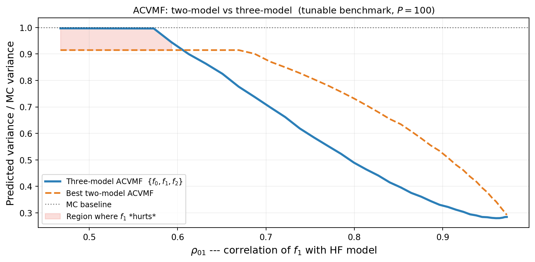
Adding a cheap LF model seems like it should always help — more data, lower cost, nothing to lose. This intuition is wrong. Consider a three-model ensemble \(\{f_0, f_1, f_2\}\) where \(f_1\) is only weakly correlated with \(f_0\). The ACV estimator must estimate control variate coefficients and allocate budget across all models. When a model contributes little variance reduction it absorbs samples that would have been better spent on the remaining models, pushing the estimator covariance above the two-model \(\{f_0, f_2\}\).
Figure 1 shows the crossover: when \(\rho_{01}\) is small the three-model estimator is worse than the best two-model subset. As \(\rho_{01}\) increases the three-model estimator eventually overtakes the two-model one.
This is not a corner case. In practice, large model libraries routinely include models that are only weakly predictive of the HF output, and naive inclusion degrades performance.
The Ensemble Selection Problem
Given a library of \(M\) candidate LF models, the ensemble selection problem is:
Find the subset \(\mathcal{M}^* \subseteq \{1, \ldots, M\}\) of LF models (always including \(f_0\)) such that the estimator using \(\{f_0\} \cup \mathcal{M}^*\) achieves the smallest predicted variance at budget \(P\).
This is a combinatorial problem: there are \(2^M\) possible subsets. For typical ensembles (\(M \leq 10\)) this is tractable — the outer enumeration over subsets is cheap because each subset’s optimal sample allocation is solved independently.
The full procedure is:
- Pilot study: evaluate all candidate models at \(N_\text{pilot}\) shared samples to estimate the joint covariance matrix.
- Enumerate subsets: for each subset of size \(\leq k\) (a user-set cap), build the estimator and optimise its sample allocation at budget \(P\).
- Select: return the subset and estimator with the smallest optimised variance.
Steps 2–3 require no additional model evaluations beyond the pilot.
The Correlation Heatmap
The joint pilot covariance (or its normalised form, the correlation matrix) is the primary diagnostic for ensemble design. Figure 2 shows the correlation matrices for two different configurations of the tunable benchmark, demonstrating how the correlation structure controls which models are worth including.

From Figure 2, the left panel shows a configuration where both LF models are useful (\(\rho_{01} = 0.96\), \(\rho_{02} = 0.41\)), while the right panel shows a case where only \(f_2\) provides meaningful correlation. Whether to include one or both LF models cannot be answered from the heatmap alone — the optimal decision also depends on model costs and the available budget.
How Many Models Is Enough?
Figure 3 shows the ACVMF variance ratio (relative to MC) for the best one-LF and two-LF subsets across a range of \(\rho_{01}\) values. The winner depends on the correlation structure: at low \(\rho_{01}\), using only \(f_2\) is best; at high \(\rho_{01}\), the full three-model ensemble wins.

In Figure 3, at low \(\rho_{01}\) the best strategy is to exclude \(f_1\) and use only \(\{f_0, f_2\}\). As \(\rho_{01}\) increases, \(f_1\) becomes valuable and the three-model ensemble dominates. The crossover point identifies the correlation threshold below which \(f_1\) should be dropped from the ensemble.
Why This Matters in Practice
Real model libraries are often assembled opportunistically: a HPC simulation suite might have a fine-mesh model, two coarse-mesh variants, a surrogate trained on a different parameter regime, and an empirical correlation. Not all of these will help. The enumeration over subsets itself is cheap (no additional model evaluations beyond the pilot), but the pilot cost grows with each model added to the library. Approaches that balance exploration of pilot statistics with exploitation of those statistics to compute the estimator are needed to determine the right number of pilot samples.
Key Takeaways
- Adding a weakly-correlated LF model can increase estimator variance relative to using a smaller ensemble (see Figure 1)
- The ensemble selection problem is: find the best subset of \(\leq k\) LF models given the pilot covariance and a target budget
- The pilot correlation heatmap (see Figure 2) is the primary visual diagnostic but is not sufficient alone — cost ratios and budget also drive the decision
- The optimal ensemble size depends on the correlation structure: stronger correlations favour larger ensembles (see Figure 3)
- Enumeration over subsets is cheap: no additional model evaluations are required beyond the pilot
Exercises
From Figure 1, at what approximate \(\rho_{01}\) does the three-model estimator break even with the best two-model subset? How does this answer depend on the budget \(P\)?
From Figure 2, in each configuration, which single LF model would you include first, and why? Would your answer change if model costs were equal?
From Figure 3, at \(\rho_{01} \approx 0.7\), the best one-LF and two-LF ensembles have similar variance. What practical consideration might break the tie in favour of fewer models?
Tip
Ready to try this? See API Cookbook → Ensemble Selection.
Next Steps
- API Cookbook —
AllSubsetsStrategy,ACVSearch, andplot_estimator_variance_reductionsin PyApprox