---
title: "Practical MCMC: Metropolis-Hastings and DRAM"
subtitle: "PyApprox Tutorial Library"
description: "Tuning proposal distributions, adaptive methods, and convergence diagnostics for MCMC."
tutorial_type: hands-on
topic: uncertainty_quantification
difficulty: intermediate
estimated_time: 12
render_time: 105
prerequisites:
- mcmc_sampling
tags:
- uq
- beam
- mcmc
- metropolis-hastings
- dram
format:
html:
code-fold: false
code-tools: true
toc: true
execute:
echo: true
warning: false
jupyter: python3
---
::: {.callout-tip collapse="true"}
## Download Notebook
[Download as Jupyter Notebook](notebooks/practical_mcmc.ipynb)
:::
## Learning Objectives
After completing this tutorial, you will be able to:
- Diagnose the effect of proposal width on chain mixing: too narrow, too wide, and well-tuned
- Use acceptance rate as a tuning diagnostic
- Explain the burn-in period and use autocorrelation to assess effective sample size
- Describe the Delayed Rejection (DR) mechanism and why it helps stuck chains
- Describe the Adaptive Metropolis (AM) mechanism and why it helps in correlated posteriors
- Use DRAM (Delayed Rejection Adaptive Metropolis) as a practical default algorithm
## Prerequisites
Complete [Sampling the Posterior with MCMC](mcmc_sampling.qmd) before this tutorial.
## Setup
We use the same KLE beam model from the [previous tutorial](mcmc_sampling.qmd): a cantilever beam whose bending stiffness $EI(x)$ varies along its length, parameterized by a 2-term KLE expansion with coefficients $\xi_1, \xi_2 \sim \mathcal{N}(0,1)$. We observe tip deflection and infer the two KLE coefficients.
```{python}
#| echo: false
import numpy as np
import matplotlib.pyplot as plt
from scipy.stats import norm
from pyapprox.util.backends.numpy import NumpyBkd
from pyapprox_benchmarks.pde.cantilever_beam import (
build_cantilever_beam_1d,
)
from pyapprox.probability.likelihood import (
DiagonalGaussianLogLikelihood,
ModelBasedLogLikelihood,
)
from pyapprox.interface.functions.fromcallable.function import (
FunctionFromCallable,
)
from pyapprox.inverse.posterior.log_unnormalized import (
LogUnNormalizedPosterior,
)
from pyapprox.inverse.sampling.metropolis import (
MetropolisHastingsSampler,
AdaptiveMetropolisSampler,
)
from pyapprox.inverse.sampling.dram import (
DelayedRejectionAdaptiveMetropolis,
)
bkd = NumpyBkd()
# 1D FEM beam with 2 KLE terms for spatially varying EI(x)
problem_2d = build_cantilever_beam_1d(bkd, num_kle_terms=2)
beam_2d = problem_2d.function() # nvars=2, nqoi=3
prior_2d = problem_2d.prior() # IndependentJoint of 2 x N(0,1)
# Tip-only wrapper (first QoI is tip deflection)
tip_model_2d = FunctionFromCallable(
nqoi=1, nvars=2,
fun=lambda xi: beam_2d(xi)[0:1, :],
bkd=bkd,
)
# True KLE parameters and synthetic data
xi_true_2d = bkd.asarray([[0.5], [-0.3]])
xi1_true = float(xi_true_2d[0, 0])
xi2_true = float(xi_true_2d[1, 0])
delta_true_2d = float(tip_model_2d(xi_true_2d)[0, 0])
sigma_noise_2d = 0.1 * abs(delta_true_2d)
noise_lik_2d = DiagonalGaussianLogLikelihood(
bkd.asarray([sigma_noise_2d**2]), bkd,
)
model_lik_2d = ModelBasedLogLikelihood(tip_model_2d, noise_lik_2d, bkd)
np.random.seed(7)
y_obs_2d = float(model_lik_2d.rvs(xi_true_2d))
noise_lik_2d.set_observations(bkd.asarray([[y_obs_2d]]))
# Posterior
posterior_2d = LogUnNormalizedPosterior(
model_fn=tip_model_2d, likelihood=noise_lik_2d, prior=prior_2d, bkd=bkd,
)
# 1D FEM beam with 1 KLE term (for the DR illustration)
problem_1d = build_cantilever_beam_1d(bkd, num_kle_terms=1)
beam_1d = problem_1d.function() # nvars=1, nqoi=3
prior_1d = problem_1d.prior()
tip_model_1d = FunctionFromCallable(
nqoi=1, nvars=1,
fun=lambda xi: beam_1d(xi)[0:1, :],
bkd=bkd,
)
xi_true_1d = 0.5
delta_true_1d = float(tip_model_1d(bkd.asarray([[xi_true_1d]]))[0, 0])
sigma_noise_1d = 0.1 * abs(delta_true_1d)
noise_lik_1d = DiagonalGaussianLogLikelihood(
bkd.asarray([sigma_noise_1d**2]), bkd,
)
model_lik_1d = ModelBasedLogLikelihood(tip_model_1d, noise_lik_1d, bkd)
np.random.seed(42)
y_obs_1d = float(model_lik_1d.rvs(bkd.asarray([[xi_true_1d]])))
noise_lik_1d.set_observations(bkd.asarray([[y_obs_1d]]))
posterior_1d = LogUnNormalizedPosterior(
model_fn=tip_model_1d, likelihood=noise_lik_1d, prior=prior_1d, bkd=bkd,
)
def run_mh(n_steps, proposal_std, seed=42):
"""Run basic MH via MetropolisHastingsSampler, return (chain, acc_rate).
Parameters
----------
n_steps : int
proposal_std : 1D array of length 2 (per-variable std devs)
seed : int
"""
np.random.seed(seed)
proposal_cov = bkd.asarray(np.diag(proposal_std**2))
sampler = MetropolisHastingsSampler(
log_posterior_fn=posterior_2d, nvars=2, bkd=bkd,
proposal_cov=proposal_cov,
)
result = sampler.sample(
nsamples=n_steps, burn=0,
initial_state=bkd.asarray([[0.0], [0.0]]),
bounds=bkd.asarray([[-4.0, 4.0], [-4.0, 4.0]]),
)
chain = bkd.to_numpy(result.samples).T # (n_steps, 2)
return chain, result.acceptance_rate
def effective_sample_size(chain_1d):
"""Estimate ESS via initial positive sequence estimator."""
n = len(chain_1d)
x = chain_1d - np.mean(chain_1d)
acf = np.correlate(x, x, mode="full")[n-1:]
acf = acf / acf[0]
# Sum autocorrelations until they go negative
tau = 1.0
for k in range(1, n // 2):
if acf[k] < 0:
break
tau += 2 * acf[k]
return n / tau
```
## Proposal Width Matters
The [previous tutorial](mcmc_sampling.qmd) used a well-tuned proposal and the chain worked. But how did we know the right proposal width? @fig-proposal-width shows what happens when the proposal is too narrow, well-tuned, and too wide.
```{python}
#| echo: false
#| fig-cap: "Effect of proposal width on chain behavior. Left: too narrow — the chain takes tiny steps and explores slowly (high acceptance, high autocorrelation). Center: well-tuned — healthy mixing, the chain moves freely through the posterior. Right: too wide — most proposals land in low-density regions and are rejected, causing the chain to stick in place for long stretches."
#| label: fig-proposal-width
from pyapprox_tutorials.figures._bayesian import plot_proposal_width
fig, axes = plt.subplots(3, 2, figsize=(13, 10))
plot_proposal_width(axes, run_mh, xi1_true, xi2_true)
plt.tight_layout()
plt.show()
```
The patterns:
- **Too narrow** (top): acceptance rate is very high ($>95\%$) because the proposals are tiny. But the chain barely moves --- it takes thousands of steps to traverse the posterior. The 2D scatter shows a tight clump rather than the full distribution.
- **Well-tuned** (middle): acceptance rate is moderate ($20\text{--}40\%$). The chain moves freely, and the 2D scatter fills out the posterior shape.
- **Too wide** (bottom): acceptance rate is very low ($<5\%$) because most proposals land far from the current position. The trace plot shows long flat stretches where the chain is stuck. The 2D scatter is sparse and clumpy.
## Acceptance Rate as a Diagnostic
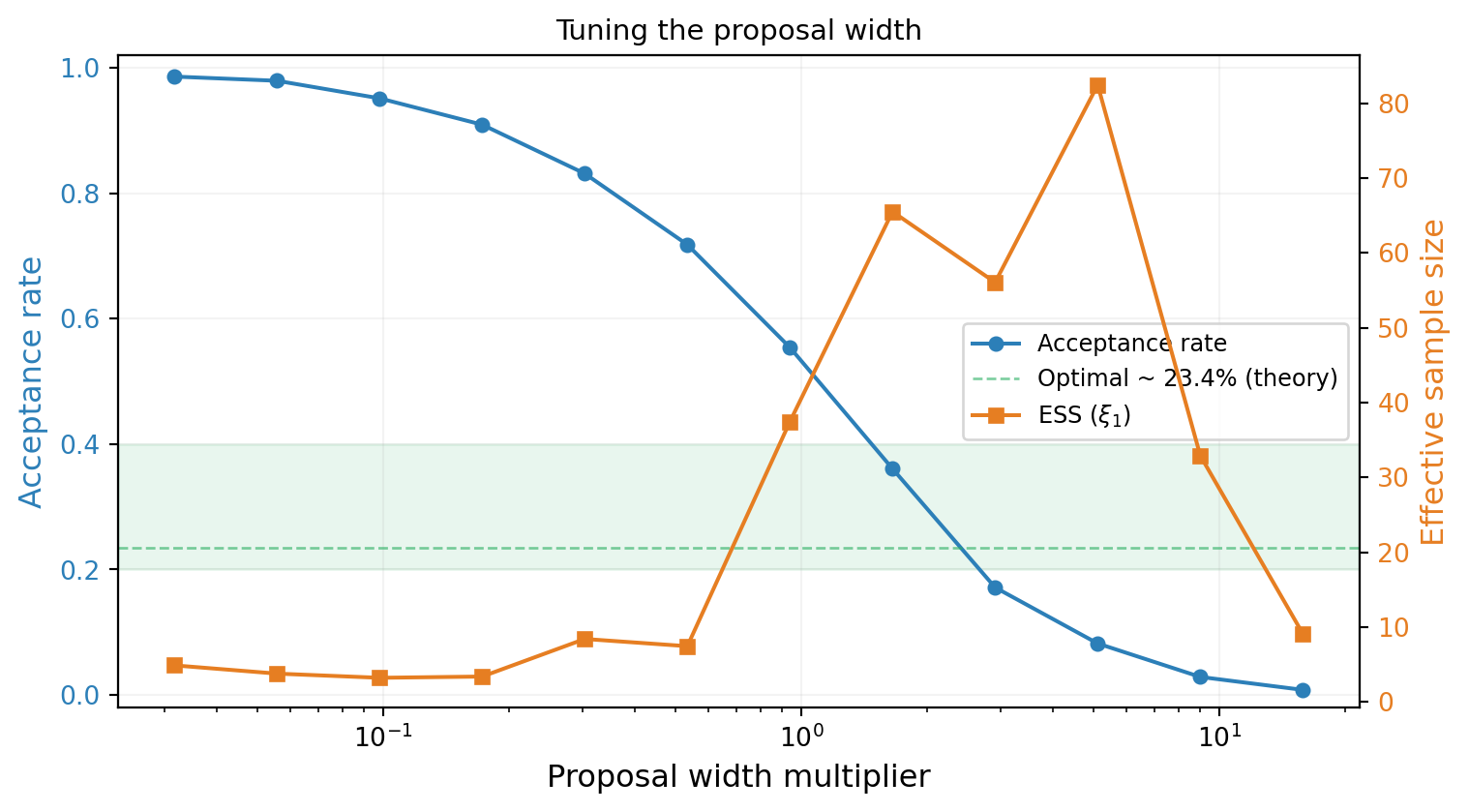
The acceptance rate provides a quick diagnostic. @fig-acceptance-rate sweeps the proposal width and plots the acceptance rate alongside the effective sample size (a measure of how many independent samples the chain produces).
```{python}
#| echo: false
#| fig-cap: "Acceptance rate and effective sample size (ESS) vs. proposal width. The optimal proposal width produces an acceptance rate of roughly $25\\text{--}40\\%$ for 2D problems. Too narrow → high acceptance but low ESS. Too wide → low acceptance and low ESS."
#| label: fig-acceptance-rate
from pyapprox_tutorials.figures._bayesian import plot_acceptance_rate
fig, ax1 = plt.subplots(figsize=(8, 4.5))
ax2 = ax1.twinx()
plot_acceptance_rate(ax1, ax2, run_mh, effective_sample_size)
plt.tight_layout()
plt.show()
```
The effective sample size peaks near the acceptance rate of $\approx 25\%$, consistent with theoretical results for random-walk Metropolis in moderate dimensions. This gives a practical rule of thumb: **tune the proposal until the acceptance rate is $20\text{--}40\%$**.
## Burn-In and Autocorrelation
### Burn-In
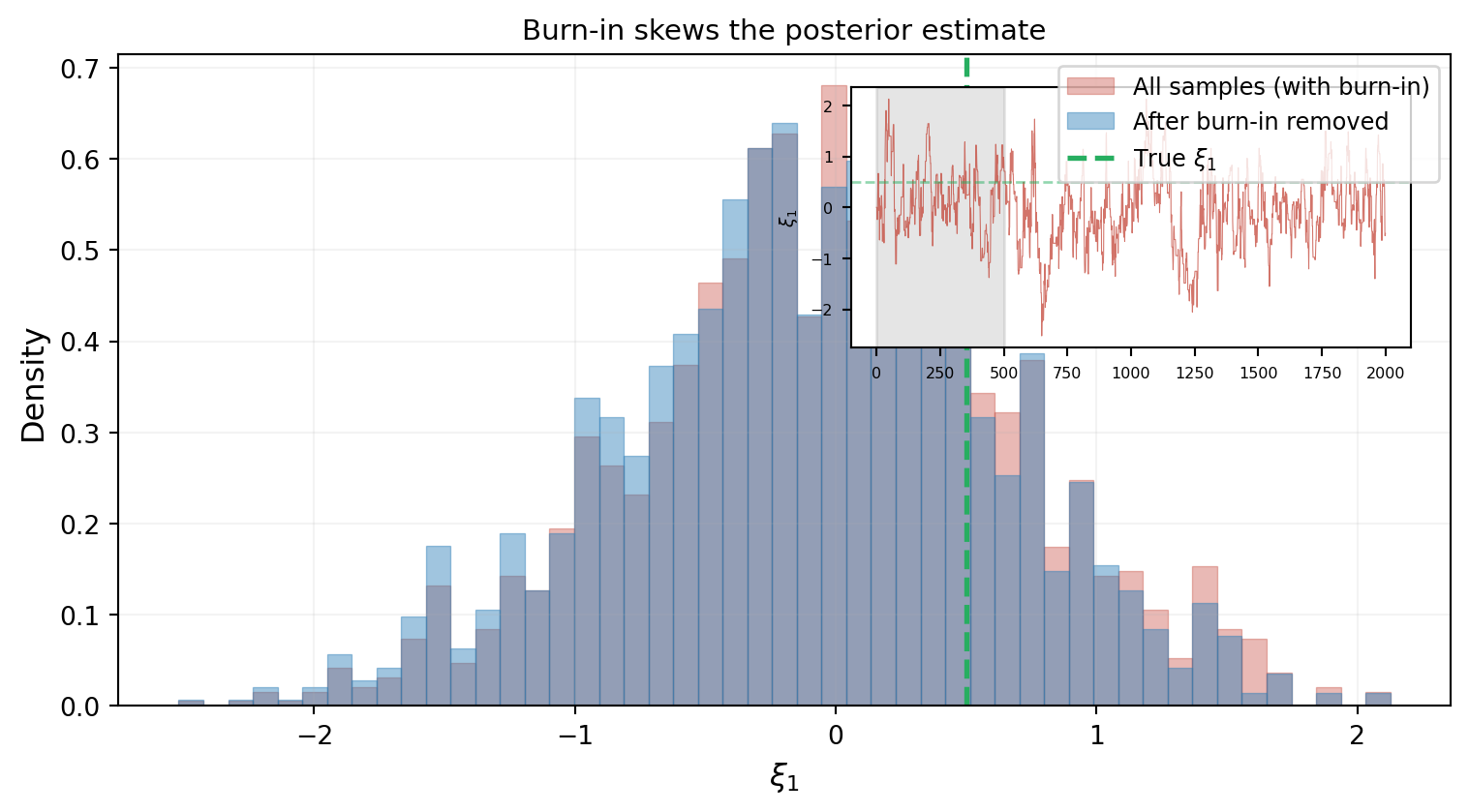
The chain starts wherever we place it and needs time to find the high-density region. Samples from this transient period are not representative of the posterior and must be discarded. This is the **burn-in** period.
@fig-burnin shows how the choice of burn-in length affects the posterior estimate.
```{python}
#| echo: false
#| fig-cap: "Effect of burn-in removal. The red histogram (all samples) is visibly shifted from the true value because the burn-in transient pulls the distribution toward the starting point. The blue histogram (burn-in removed) centers on the true value. The inset trace plot shows the transient approach phase (gray region)."
#| label: fig-burnin
from pyapprox_tutorials.figures._bayesian import plot_burnin
fig, ax = plt.subplots(figsize=(8, 4.5))
plot_burnin(ax, run_mh, xi1_true)
plt.tight_layout()
plt.show()
```
### Autocorrelation
Even after burn-in, consecutive chain samples are correlated --- the walker's position at step $t$ depends on where it was at step $t-1$. The **autocorrelation function** measures how quickly this dependence decays.
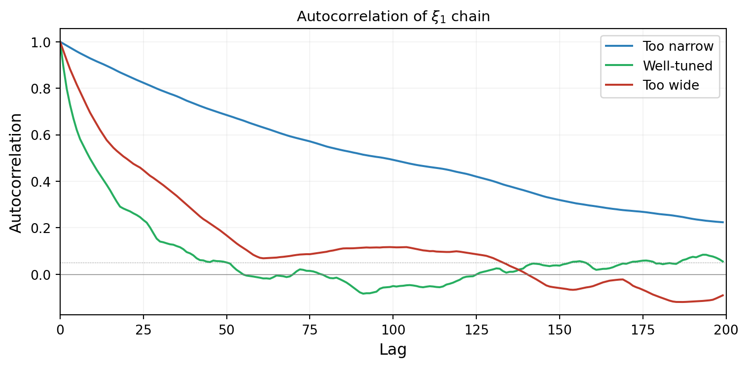
@fig-autocorrelation compares the autocorrelation for the three proposal widths. A well-tuned chain decorrelates quickly; a poorly tuned chain stays correlated for many steps.
```{python}
#| echo: false
#| fig-cap: "Autocorrelation of the $\\xi_1$ chain for three proposal widths. The well-tuned chain (green) decorrelates within ~20 steps. The too-narrow chain (blue) stays correlated for hundreds of steps. The too-wide chain (red) also decorrelates slowly due to frequent rejections."
#| label: fig-autocorrelation
from pyapprox_tutorials.figures._bayesian import plot_autocorrelation
configs = [
{"sigma": np.array([0.05, 0.05]), "label": "Too narrow", "color": "#2C7FB8"},
{"sigma": np.array([0.5, 0.5]), "label": "Well-tuned", "color": "#27AE60"},
{"sigma": np.array([5.0, 5.0]), "label": "Too wide", "color": "#C0392B"},
]
fig, ax = plt.subplots(figsize=(8, 4))
plot_autocorrelation(ax, run_mh, configs)
plt.tight_layout()
plt.show()
```
## Delayed Rejection (DR)
Standard Metropolis-Hastings has a binary outcome: accept or reject. If a proposal is rejected, the chain stays at the current position and tries again from scratch. This is wasteful --- the rejected proposal told us that the proposed *direction* might be fine, but the *step was too large*.
**Delayed Rejection** adds a second chance: if the first proposal is rejected, try a second proposal with a **smaller step size**. The acceptance probability for the second stage is adjusted to maintain the correct stationary distribution.
@fig-delayed-rejection illustrates the mechanism on the 1D KLE beam posterior.
```{python}
#| echo: false
#| fig-cap: "Delayed Rejection in action. Top: the first proposal (large step) lands in a low-density region and is rejected. Bottom: a second proposal (smaller step) is tried from the same current position. It lands in a higher-density region and is accepted. Without DR, the chain would have stayed put."
#| label: fig-delayed-rejection
from pyapprox_tutorials.figures._bayesian import plot_delayed_rejection
fig, (ax1, ax2) = plt.subplots(2, 1, figsize=(9, 6), sharex=True)
plot_delayed_rejection(ax1, ax2, tip_model_1d, y_obs_1d, sigma_noise_1d,
bkd)
plt.tight_layout()
plt.show()
```
The key idea: **DR gives the chain a second chance with a more conservative step**, preventing it from getting stuck after an aggressive proposal is rejected. This is especially useful when the posterior has regions of very different curvature.
## Adaptive Metropolis (AM)
Standard Metropolis-Hastings uses a fixed proposal distribution. But the optimal proposal depends on the posterior's shape, which we don't know in advance. **Adaptive Metropolis** solves this by learning the proposal covariance from the chain history:
$$
\mathbf{C}_{\text{prop}}^{(t)} = s_d \cdot \hat{\boldsymbol{\Sigma}}_t + \varepsilon \mathbf{I}
$$
where $\hat{\boldsymbol{\Sigma}}_t$ is the sample covariance of the chain so far, $s_d = 2.4^2 / d$ is a scaling factor, and $\varepsilon \mathbf{I}$ is a small regularization term.
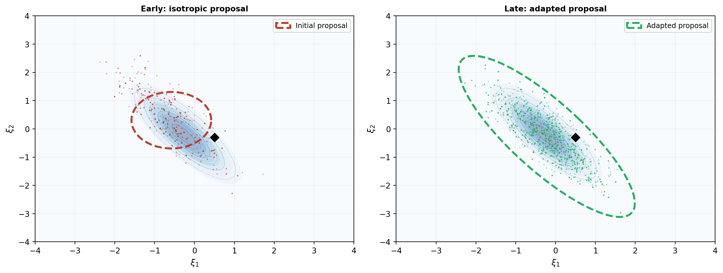
@fig-adaptive-proposal shows the effect on the KLE beam problem. Initially the proposal is isotropic (circular). As the chain runs, the proposal adapts to match the posterior's elongated shape.
```{python}
#| echo: false
#| fig-cap: "Adaptive Metropolis learns the posterior shape. Left: initial isotropic proposal (circle) — the chain makes many rejected moves perpendicular to the posterior ridge. Right: after adaptation, the proposal aligns with the posterior's correlation structure (tilted ellipse) — the chain moves efficiently along the ridge."
#| label: fig-adaptive-proposal
from pyapprox_tutorials.figures._bayesian import plot_adaptive_proposal
# Run adaptive MH
n_steps_am = 3000
initial_cov = bkd.asarray([[0.5**2, 0.0], [0.0, 0.5**2]])
cov_early = bkd.to_numpy(initial_cov)
sampler_am = AdaptiveMetropolisSampler(
log_posterior_fn=posterior_2d, nvars=2, bkd=bkd,
proposal_cov=initial_cov,
adaptation_start=200, adaptation_interval=50,
)
np.random.seed(42)
result_am = sampler_am.sample(
nsamples=n_steps_am, burn=0,
initial_state=bkd.asarray([[0.0], [0.0]]),
bounds=bkd.asarray([[-4.0, 4.0], [-4.0, 4.0]]),
)
chain_am = bkd.to_numpy(result_am.samples).T
acc_am = result_am.acceptance_rate
cov_late = bkd.to_numpy(sampler_am.proposal_covariance())
fig, (ax1, ax2) = plt.subplots(1, 2, figsize=(13, 5))
plot_adaptive_proposal(ax1, ax2, chain_am, cov_early, cov_late,
posterior_2d, xi1_true, xi2_true, bkd)
plt.tight_layout()
plt.show()
```
The adapted proposal ellipse is tilted to align with the posterior's correlation between $\xi_1$ and $\xi_2$. This means the chain proposes moves *along* the high-density ridge rather than *across* it, dramatically improving mixing.
## DRAM: Combining DR and AM
**DRAM** (Delayed Rejection Adaptive Metropolis) combines both ideas:
- **Adaptive Metropolis** learns the proposal shape from the chain → efficient moves along the posterior ridge
- **Delayed Rejection** provides a fallback when an adaptive proposal is rejected → the chain unsticks faster
@fig-dram-comparison compares the four methods on the KLE beam problem. All chains use the same number of steps and start from the same initial point.
```{python}
#| echo: false
#| fig-cap: "Comparison of four MCMC variants on the KLE beam problem (3,000 steps each). Top row: trace plots of $\\xi_1$. Bottom row: 2D scatter of posterior samples with ESS annotations. Focus on ESS rather than acceptance rate — DR achieves 90% acceptance but the lowest ESS, because most accepted moves are tiny second-stage steps that barely advance the chain."
#| label: fig-dram-comparison
from pyapprox_tutorials.figures._bayesian import plot_dram_comparison
n_compare = 3000
burnin_comp = 500
initial_cov_comp = bkd.asarray([[0.5**2, 0.0], [0.0, 0.5**2]])
# MH: fixed proposal
chain_mh, acc_mh = run_mh(n_compare, np.array([0.5, 0.5]), seed=42)
# AM: already computed above
chain_am_c = chain_am
# DR: DRAM with adaptation disabled (adaptation_start set very high)
sampler_dr = DelayedRejectionAdaptiveMetropolis(
log_posterior_fn=posterior_2d, nvars=2, bkd=bkd,
proposal_cov=initial_cov_comp,
adaptation_start=999999, adaptation_interval=50,
dr_scale=0.1,
)
np.random.seed(42)
result_dr = sampler_dr.sample(
nsamples=n_compare, burn=0,
initial_state=bkd.asarray([[0.0], [0.0]]),
bounds=bkd.asarray([[-4.0, 4.0], [-4.0, 4.0]]),
)
chain_dr = bkd.to_numpy(result_dr.samples).T
acc_dr = result_dr.acceptance_rate
# DRAM: full delayed rejection + adaptive
sampler_dram = DelayedRejectionAdaptiveMetropolis(
log_posterior_fn=posterior_2d, nvars=2, bkd=bkd,
proposal_cov=initial_cov_comp,
adaptation_start=200, adaptation_interval=50,
dr_scale=0.1,
)
np.random.seed(42)
result_dram = sampler_dram.sample(
nsamples=n_compare, burn=0,
initial_state=bkd.asarray([[0.0], [0.0]]),
bounds=bkd.asarray([[-4.0, 4.0], [-4.0, 4.0]]),
)
chain_dram = bkd.to_numpy(result_dram.samples).T
acc_dram = result_dram.acceptance_rate
methods = [
("MH", chain_mh, acc_mh, "#2C7FB8"),
("AM", chain_am_c, acc_am, "#E67E22"),
("DR", chain_dr, acc_dr, "#8E44AD"),
("DRAM", chain_dram, acc_dram, "#27AE60"),
]
fig, axes = plt.subplots(2, 4, figsize=(16, 7))
plot_dram_comparison(axes, methods, xi1_true, xi2_true,
effective_sample_size, burnin_comp=burnin_comp)
plt.tight_layout()
plt.show()
```
Several observations:
- **DR** achieves the highest acceptance rate (~90%) but the *lowest* ESS. Its second-stage proposals are small, so most accepted DR moves barely advance the chain. High acceptance rate is misleading here.
- **AM** achieves the real improvement by learning the posterior's correlation structure. Its ESS is dramatically higher than both MH and DR.
- **DRAM** combines both mechanisms, matching or exceeding AM's efficiency on this near-Gaussian posterior while providing a safety net for harder problems where the adapted proposal occasionally proposes too aggressively.
For most problems, **DRAM is a good default choice** — it is at least as good as AM and more robust on non-Gaussian posteriors.
## Practical Guidance
Based on what we've seen:
1. **Start with DRAM** unless you have a reason to use something simpler.
2. **Check the acceptance rate**: aim for $20\text{--}40\%$ for standard MH and AM in moderate dimensions. DR and DRAM will report higher rates because the second-stage proposals recover first-stage rejections — focus on ESS rather than acceptance rate for these methods.
3. **Inspect trace plots**: look for the chain settling into a stationary pattern. Flat stretches indicate the chain is stuck.
4. **Remove burn-in**: discard the initial transient. When in doubt, be generous --- discarding too many samples is safer than including biased ones.
5. **Check autocorrelation**: if the chain is highly correlated, you need a longer run to get enough effective samples.
6. **Run multiple chains** from different starting points. If they converge to the same distribution, this is strong evidence that the chains have mixed properly.
::: {.callout-note}
## When MCMC is too expensive
Each MCMC step requires one model evaluation. For this 1D cantilever beam with a fast FEM solver, 3,000 evaluations are trivial. But for a 3D FEM model that takes minutes per evaluation, 5,000 evaluations is prohibitive. In such cases, replacing the expensive model with a polynomial chaos surrogate inside the MCMC loop can reduce the cost by orders of magnitude.
:::
## Key Takeaways
- **Proposal width** controls chain behavior: too narrow → slow exploration; too wide → frequent rejection; well-tuned → efficient mixing
- The **acceptance rate** is a quick diagnostic: aim for $20\text{--}40\%$ in moderate dimensions
- **Burn-in** must be removed; **autocorrelation** determines the effective sample size
- **Delayed Rejection (DR)** gives the chain a second chance with a smaller step when the first proposal is rejected
- **Adaptive Metropolis (AM)** learns the proposal covariance from the chain history, aligning the proposal with the posterior shape
- **DRAM** combines both and is a good default for most problems
## Exercises
1. Run standard MH on the KLE beam with acceptance rates of 10%, 25%, and 50% (adjust proposal width to achieve each). Compare the effective sample size. Which is best?
2. Modify the DR implementation to use three stages instead of two (a third, even smaller proposal). Does the acceptance rate improve? Does the effective sample size change?
3. In the AM algorithm, the adaptation starts after 200 steps (`adaptation_start = 200`). What happens if you start adapting immediately ($t = 1$)? What if you wait until $t = 1000$? Why does the choice matter?
4. **(Challenge)** Add a second observation (stress measurement in addition to deflection) to the 2D problem. How does the posterior shape change? Does DRAM still outperform standard MH?