Multilevel Best Linear Unbiased Estimators
PyApprox Tutorial Library
How viewing multi-fidelity estimation as a generalized least-squares problem over flexible model subsets produces an estimator that reaches the multi-model CV ceiling — without requiring a hierarchical correction chain.
TipDownload Notebook
Learning Objectives
After completing this tutorial, you will be able to:
- Explain how MLBLUE frames multi-fidelity estimation as generalized least squares rather than a control-variate correction
- Describe what a subset is and how the subset design determines which models are co-evaluated on shared sample points
- Interpret the restriction matrix \(\mathbf{H}\), the error covariance \(\mathbf{C}_{\boldsymbol{\epsilon}\boldsymbol{\epsilon}}\), and the observation vector \(\mathbf{Y}\)
- State the key convergence property: MLBLUE reaches the multi-model CV ceiling while MLMC and MFMC are permanently capped at CV-1
- Identify when MLBLUE’s unrestricted subset design is an advantage over the ACV family
Prerequisites
Complete General ACV Concept before this tutorial. MLBLUE reaches the same variance floor as ACVMF but through an entirely different framing — understanding both is valuable when either does not map naturally onto the problem structure.
A Different Angle on Multi-Fidelity Estimation
Every estimator so far corrects a noisy HF mean estimate using cheap LF correction terms. MLBLUE takes a completely different angle: it jointly estimates the means of all models simultaneously using generalized least squares (GLS), then extracts the HF mean as a linear combination of the full joint estimate.
The structural choice in MLBLUE is not an allocation matrix or a recursion index — it is a set of subsets. A subset \(S_k \subseteq \{0, 1, \ldots, M\}\) is any non-empty collection of model indices. For each subset you draw \(m_k\) independent samples and evaluate every model in \(S_k\) at each of those sample points. There is no requirement that subsets form a chain, star, or any particular nesting pattern.
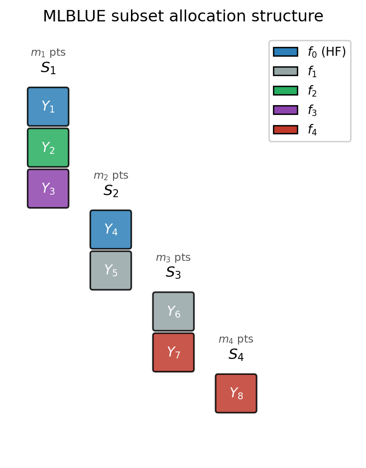
Subsets and the Observation Vector
Figure 1 shows the subset structure for a three-model example with four active subsets. Each column is one subset; stacked coloured blocks show which models are evaluated at the same \(m_k\) sample points.
Reading Figure 1: the leftmost column co-evaluates three models (\(f_0, f_2, f_3\)) and produces stacked observations \(Y_1, Y_2, Y_3\). The rightmost column at bottom is a cheap singleton (\(f_4\)) that evaluates only the cheapest model alone — accumulating many inexpensive samples that still contribute useful information about the joint mean vector through the GLS system.
Assembling the Least-Squares System
Each observation at a sample \(\boldsymbol{\theta}_k^{(i)}\) within subset \(k\) satisfies: \[ \mathbf{Y}_k^{(i)} = \mathbf{R}_k\,\mathbf{q} + \boldsymbol{\epsilon}_k^{(i)}, \] where \(\mathbf{q} = [Q_0, \ldots, Q_M]^\top\) are all model means (the unknowns), \(\mathbf{R}_k \in \{0,1\}^{|S_k|\times(M+1)}\) is the restriction operator whose row \(\ell\) has a single 1 in the column of the \(\ell\)-th model in \(S_k\), and \(\boldsymbol{\epsilon}_k^{(i)}\) is zero-mean noise. Stacking all subsets and samples gives the full system \(\mathbf{Y} = \mathbf{H}\mathbf{q} + \boldsymbol{\epsilon}\).
Figure 2 shows this construction for three active subsets with small sample counts.
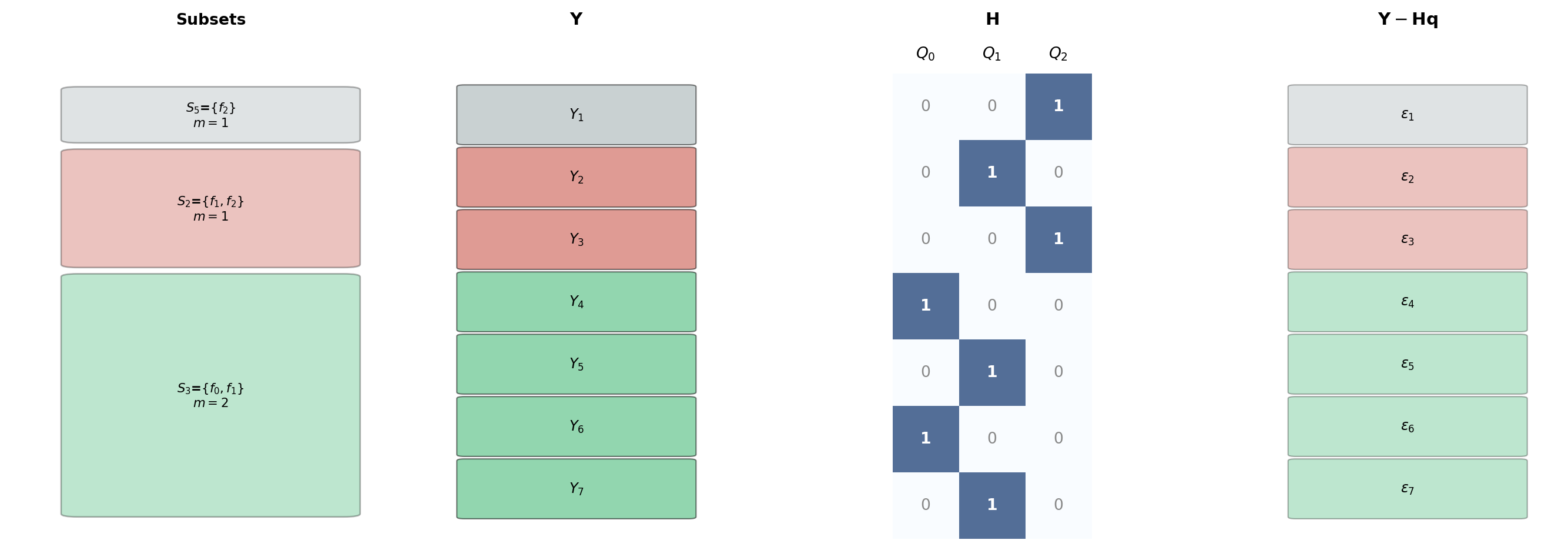
Three things to notice in Figure 2:
- Row count equals total evaluations. \(\mathbf{H}\) has one row per model evaluation across all subsets and all samples: \(\sum_k m_k |S_k|\) rows total.
- Column count equals number of model means. Three columns for three means (\(Q_0, Q_1, Q_2\)).
- Repeated subset samples contribute identical row blocks. The two samples of \(S_3\) produce four rows but each pair is structurally identical — only the data values differ.
The Error Covariance
Models within the same subset, evaluated at the same sample point, are correlated. The full error covariance is block-diagonal: \[ \mathbf{C}_{\boldsymbol{\epsilon}\boldsymbol{\epsilon}} = \mathrm{BlockDiag}(G_1, \ldots, G_K), \qquad G_k = \mathrm{BlockDiag}(\underbrace{C_k, \ldots, C_k}_{m_k}), \] where \(C_k = \mathbf{R}_k\,\boldsymbol{\Sigma}\,\mathbf{R}_k^\top\) is the submatrix of the population covariance \(\boldsymbol{\Sigma}\) for the models in \(S_k\), estimated from the pilot study. Figure 3 shows this block structure for the same three-subset example.
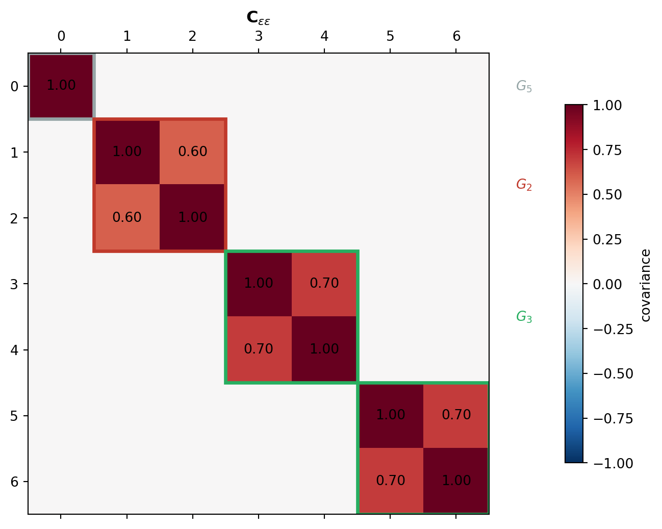
Because \(\mathbf{C}_{\boldsymbol{\epsilon}\boldsymbol{\epsilon}}\) is block-diagonal, its inverse is also block-diagonal and the GLS problem reduces to the tractable normal equations \[ \boldsymbol{\Psi}\,\mathbf{q}^B = \mathbf{y}, \qquad \boldsymbol{\Psi} = \sum_{k=1}^K m_k\,\mathbf{R}_k^\top C_k^{-1} \mathbf{R}_k, \qquad \mathbf{y} = \sum_{k=1}^K \mathbf{R}_k^\top C_k^{-1}\! \sum_{i=1}^{m_k} \mathbf{Y}_k^{(i)}. \]
The MLBLUE estimator \(\mathbf{q}^B = \boldsymbol{\Psi}^{-1}\mathbf{y}\) is unbiased for \(\mathbf{q}\) and has variance \(\mathbb{V}[Q^B_\beta] = \boldsymbol{\beta}^\top\boldsymbol{\Psi}^{-1}\boldsymbol{\beta}\) for any target vector \(\boldsymbol{\beta}\). Setting \(\boldsymbol{\beta} = \mathbf{e}_0\) extracts the HF mean estimate.
Convergence to the Multi-Model CV Ceiling
Like ACVMF, MLBLUE converges to the multi-model CV ceiling as LF sample counts grow. MLMC and MFMC plateau at the CV-1 ceiling. Figure 4 demonstrates this by fixing the HF sample count at \(N_0 = 1\) and steadily increasing LF samples on the five-model polynomial benchmark.
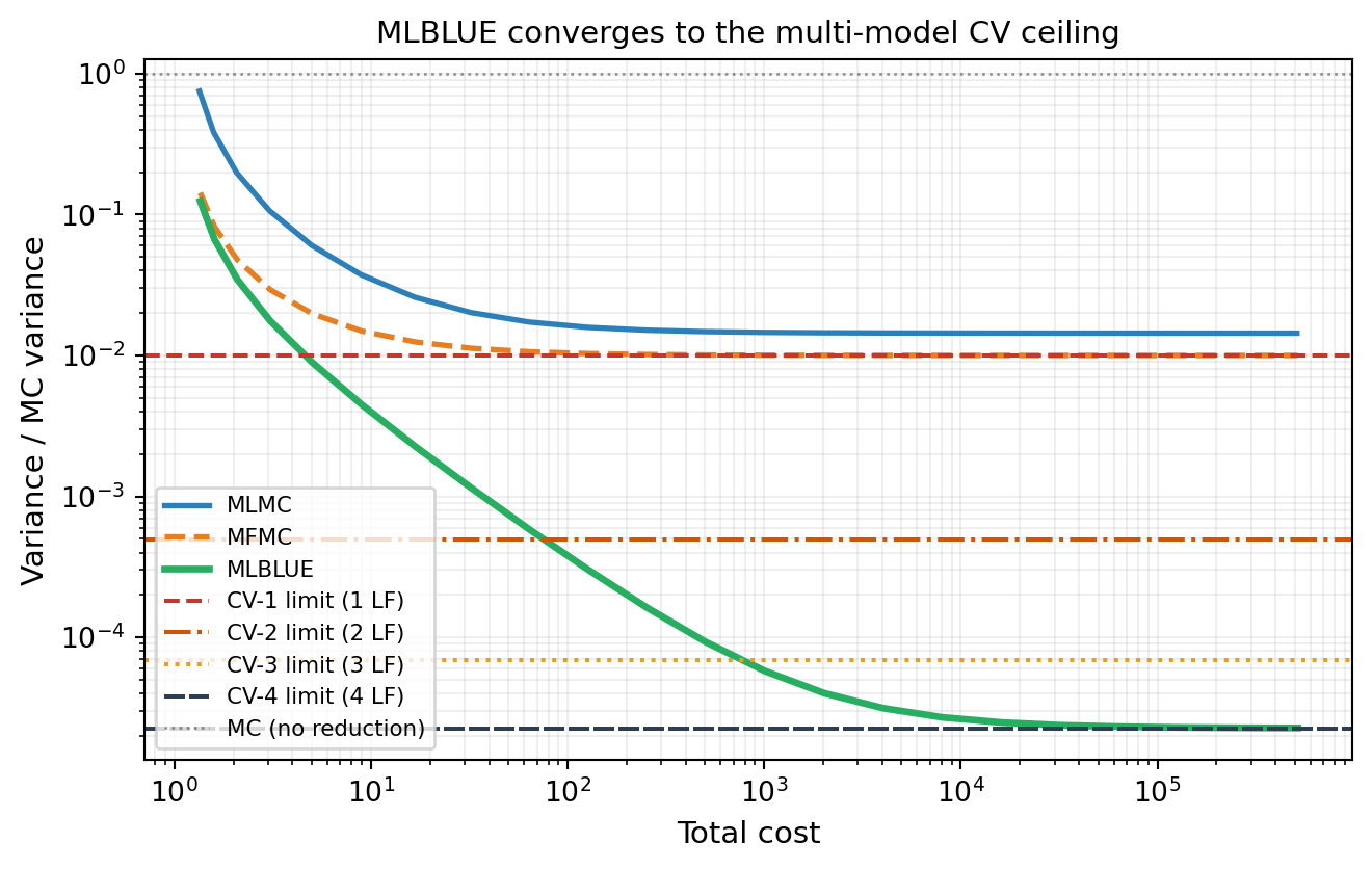
The convergence is structural: \(\boldsymbol{\Psi}\) aggregates information from every subset simultaneously. As LF sample counts grow, every LF mean \(Q_j\) is estimated with negligible error, and the GLS estimator for \(Q_0\) saturates at the CV-\(M\) lower bound. MLMC and MFMC cannot achieve this because only the one-step correction \(\Delta_1\) directly reduces variance for \(Q_0\).
Key Takeaways
- MLBLUE estimates all model means jointly via GLS; the HF mean is extracted via \(Q^B_0 = \boldsymbol{e}_0^\top\mathbf{q}^B\)
- Subsets define co-evaluation groups; any non-empty subsets are valid — no chain or nesting required (see Figure 1)
- Three ingredients: restriction operator \(\mathbf{R}_k\) (who is measured), per-subset error covariance \(C_k\) (how correlated), block-diagonal \(\mathbf{C}_{\boldsymbol{\epsilon}\boldsymbol{\epsilon}}\) (across all subsets and samples) (see Figure 2, Figure 3)
- Like ACVMF, MLBLUE converges to CV-\(M\) and is not capped at CV-1 (see Figure 4)
- The subset design is most flexible when physically incompatible models prevent certain co-evaluations
Exercises
In Figure 1, how many evaluations does the leftmost subset contribute to \(\mathbf{Y}\)? What is the total length of \(\mathbf{Y}\) across all shown subsets (assume \(m_k = 1\) for each)?
From Figure 2, how many rows does \(\mathbf{H}\) have? How many columns? What does each column correspond to?
From Figure 3, why is \(G_3\) a \(2\times 2\) matrix while \(G_5\) is \(1\times 1\)? Why does \(G_3\) appear twice but \(G_2\) appears once?
Suppose \(f_0\) and \(f_2\) cannot be co-evaluated. Which subsets must be excluded? Can MLBLUE still use \(f_2\) to improve the HF mean estimate?
From Figure 4: at sample ratio \(r = 100\), how much better is MLBLUE than MLMC? Estimate as a ratio of variance reductions.
Next Steps
- MLBLUE Analysis — Formal derivation of \(\boldsymbol{\Psi}\), the variance formula, and its connection to the CV-\(M\) limit
- API Cookbook — Define subsets, run MLBLUE end-to-end, compare to MLMC and PACV in PyApprox
Tip
Ready to try this? See API Cookbook → MLBLUEEstimator.
References
[SUSIAMUQ2020] D. Schaden, E. Ullmann. On multilevel best linear unbiased estimators. SIAM/ASA J. Uncertainty Quantification 8(2):601–635, 2020. DOI
[SUSIAMUQ2021] D. Schaden, E. Ullmann. Asymptotic Analysis of Multilevel Best Linear Unbiased Estimators. SIAM/ASA J. Uncertainty Quantification 9(3):953–978, 2021. DOI
[CWARXIV2023] M. Croci, K. Willcox, S. Wright. Multi-output multilevel best linear unbiased estimators via semidefinite programming. Computer Methods in Applied Mechanics and Engineering, 2023. DOI