import numpy as np
import matplotlib.pyplot as plt
from pyapprox.util.backends.numpy import NumpyBkd
from pyapprox_benchmarks.expdesign.linear_gaussian import (
    build_linear_gaussian_kl_benchmark,
)
from pyapprox.expdesign.data import generate_oed_data
from pyapprox.expdesign.diagnostics import (
    KLOEDDiagnostics,
    compute_convergence_rate,
    compute_estimator_mse,
)
from pyapprox.expdesign.quadrature import HaltonSampler, MonteCarloSampler
from pyapprox.expdesign.quadrature.oed import (
    OEDQuadratureSampler,
    build_oed_joint_distribution,
)

np.random.seed(1)
bkd = NumpyBkd()Bayesian OED: Verifying Convergence with KLOEDDiagnostics
PyApprox Tutorial Library
Using KLOEDDiagnostics to measure MSE, decompose bias and variance, and confirm that the outer sample count drives convergence.
TipDownload Notebook
Learning Objectives
After completing this tutorial, you will be able to:
- Construct a linear Gaussian KL-OED benchmark and query its exact EIG
- Use
KLOEDDiagnosticswith manually generated samples to estimate EIG - Decompose total MSE into squared bias and variance using
compute_estimator_mse - Confirm empirically that outer sample count \(M\) drives variance while inner count \(N_\text{in}\) drives bias
- Read convergence rates from
compute_convergence_rateand match them to theory
Prerequisites
Complete The Double-Loop Estimator before this tutorial. The estimator has two sample budgets: outer (\(M\)) controls variance; inner (\(N_\text{in}\)) controls the bias from the evidence approximation. We verify both empirically here.
Setup
# Problem parameters — match test_kl_oed_convergence.py for reproducibility
nobs      = 5
degree    = 2
noise_std = 0.5
prior_std = 0.5

benchmark = build_linear_gaussian_kl_benchmark(nobs, degree, noise_std, prior_std, bkd)
problem   = benchmark.problem()
nparams   = problem.nparams()

# Uniform design: equal weight on every candidate observation
weights = bkd.ones((nobs, 1)) / nobs
The diagnostics API separates sampling from estimation. OEDQuadratureSampler draws joint (prior + noise) samples from a single low-discrepancy sequence, and generate_oed_data evaluates the forward map on those samples:
joint_dist = build_oed_joint_distribution(problem, bkd)

def make_mc_sampler(seed):
    """Create a MonteCarloSampler for the joint distribution."""
    np.random.seed(seed)
    return OEDQuadratureSampler(
        MonteCarloSampler(joint_dist, bkd), nparams, bkd,
    )
Exact EIG as Ground Truth
The benchmark provides a closed-form EIG for any design weights, giving us an exact reference against which to measure numerical error.
exact = benchmark.exact_eig(weights)A single numerical estimate with moderate sample counts:
noise_variances = bkd.full((nobs,), noise_std**2)
diagnostics = KLOEDDiagnostics(noise_variances, bkd)

data = generate_oed_data(
    problem, make_mc_sampler(42), make_mc_sampler(5042), 200, 100,
)
approx = diagnostics.compute_numerical_eig(
    weights, data.outer_shapes, data.latent_samples, data.inner_shapes,
)
TipReproducibility
Sampling is fully reproducible when using a fixed seed in make_mc_sampler. Always record your seed alongside results so experiments can be re-run exactly.
MSE Decomposition: Bias and Variance
We run nrealizations independent estimates and decompose total MSE into squared bias and variance: \(\text{MSE} = \text{bias}^2 + \text{variance}\).
def compute_eig_realization(nouter, ninner, seed):
    data = generate_oed_data(
        problem, make_mc_sampler(seed), make_mc_sampler(seed + 5000),
        nouter, ninner,
    )
    return diagnostics.compute_numerical_eig(
        weights, data.outer_shapes, data.latent_samples, data.inner_shapes,
    )

estimates = [compute_eig_realization(100, 50, seed=s) for s in range(20)]
bias, variance, mse = compute_estimator_mse(exact, estimates)
Outer vs. Inner: Which Budget Matters More?
The two figures below answer this directly. The left panel sweeps \(M\) (outer samples) with fixed \(N_\text{in}\), showing how MSE decays with the outer budget. The right panel sweeps \(N_\text{in}\) (inner samples) with fixed \(M\), showing how bias² and variance each respond to the inner budget.
outer_counts = [100, 250, 500, 1000, 2000]
inner_counts = [50, 200]
M_fixed      = 500
inner_sweep  = [5, 10, 25, 50, 100, 200]
nrealizations = 30

def sweep_mse(outer_list, inner_list):
    """Compute MSE grid over outer x inner sample counts."""
    all_mse, all_sqbias, all_var = [], [], []
    for ninner in inner_list:
        mse_row, sqbias_row, var_row = [], [], []
        for nouter in outer_list:
            ests = [compute_eig_realization(nouter, ninner, seed=s)
                    for s in range(nrealizations)]
            b, v, m = compute_estimator_mse(exact, ests)
            mse_row.append(m)
            sqbias_row.append(b**2)
            var_row.append(v)
        all_mse.append(bkd.asarray(mse_row))
        all_sqbias.append(bkd.asarray(sqbias_row))
        all_var.append(bkd.asarray(var_row))
    return {"mse": all_mse, "sqbias": all_sqbias, "variance": all_var}

# Outer sweep
values_mc = sweep_mse(outer_counts, inner_counts)

# Inner sweep: fix M, vary N_in
values_inner = sweep_mse([M_fixed], inner_sweep)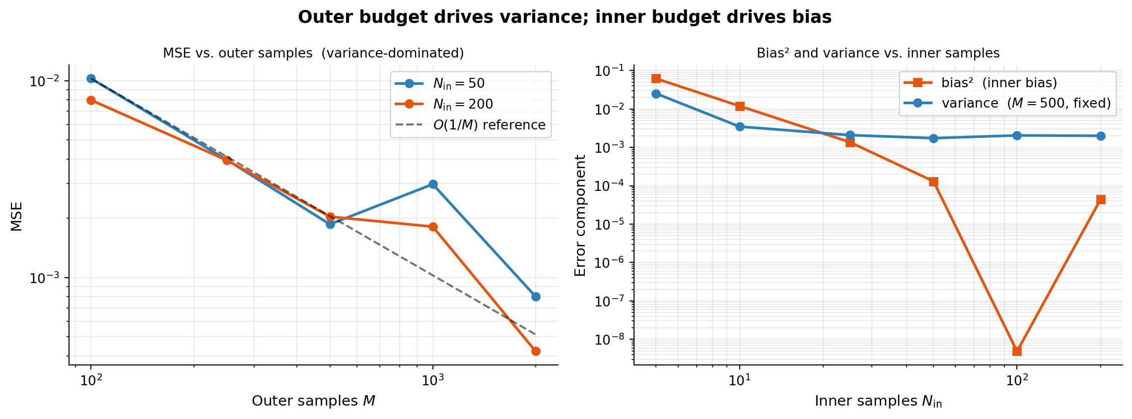
# Convergence rates
for ii, ninner in enumerate(inner_counts):
    rate = compute_convergence_rate(
        outer_counts,
        bkd.to_numpy(values_mc["mse"][ii]).tolist(),
    )
A rate near 1.0 confirms the \(O(1/M)\) variance decay. The right panel shows bias² falling steeply once \(N_\text{in} \gtrsim 50\), after which MSE is dominated by variance from the outer loop. Increasing \(N_\text{in}\) beyond that point yields diminishing returns — invest budget in \(M\) instead.
For faster convergence with the same \(M\), see MC vs. Halton for EIG Estimation.
Key Takeaways
build_linear_gaussian_kl_benchmarkprovides an exact EIG reference for any weights.- The caller generates samples and passes raw arrays to
KLOEDDiagnostics— this separation makes it easy to swap MC for QMC or other sampling strategies. compute_estimator_msedecomposes total MSE into squared bias and variance across independent realizations.- The outer sample count \(M\) controls variance and follows \(O(1/M)\); the inner count \(N_\text{in}\) controls bias, which becomes negligible once \(N_\text{in} \gtrsim 50\) for this problem.
- Once bias² is small relative to variance, further increasing \(N_\text{in}\) wastes compute — increase \(M\) instead.
Exercises
Run the MSE decomposition with
nouter=50, ninner=5and compare bias² to variance. At this extreme, which term dominates?From the right panel, estimate the convergence rate of bias² with respect to \(N_\text{in}\). Is it faster or slower than the \(O(1/M)\) outer rate? Why?
Try
degree=4(more parameters). Does the exact EIG increase or decrease relative todegree=2? Does the \(N_\text{in}\) needed to suppress bias change?
Next Steps
- MC vs. Halton for EIG Estimation — achieving faster convergence by replacing Monte Carlo with quasi-random sequences
- Goal-Oriented Bayesian OED — when prediction accuracy matters more than parameter estimation