
Sampling the Posterior with MCMC
PyApprox Tutorial Library
Using Markov chain Monte Carlo to generate posterior samples when grid evaluation is infeasible.
TipDownload Notebook
Learning Objectives
After completing this tutorial, you will be able to:
- Explain why grid evaluation of the posterior fails in more than one or two dimensions
- Describe the core idea of MCMC: a random walker that preferentially visits high-density regions
- Trace through the propose-then-accept/reject mechanism on a simple example
- Run MCMC on a 1D problem and verify it recovers the exact posterior
- Extend MCMC to a 2D problem and inspect the chain’s trajectory
- Perform a posterior predictive check to verify inference is consistent with the data
Prerequisites
Complete From Data to Parameters: Introduction to Bayesian Inference before this tutorial.
The Grid Breaks Down
The previous tutorial computed the posterior exactly by evaluating the prior \(\times\) likelihood on a grid of 500 points. With one parameter, this required 500 model evaluations — entirely feasible.
But the cost of a grid grows exponentially with the number of parameters:
| Parameters | Grid points (\(500^d\)) | Model evaluations |
|---|---|---|
| 1 | 500 | 500 |
| 2 | 250,000 | 250,000 |
| 3 | 125,000,000 | 125,000,000 |
| 5 | \(3.1 \times 10^{13}\) | impossible |
Even for a 2-parameter beam, a grid requires 250,000 model solves. We need an approach that generates samples from the posterior without evaluating it everywhere.
The Random Walk Idea
Imagine placing a walker at some starting location in parameter space. At each step, the walker:
- Proposes a random move (e.g., a small step in a random direction)
- Evaluates whether the new location has higher or lower posterior density
- Decides whether to accept the move or stay put
If the walker always accepts moves to higher density and sometimes accepts moves to lower density, it will spend most of its time in the high-density regions of the posterior — which is exactly where we need samples.
Figure 1 shows this on a 2D posterior. The walker’s trajectory traces out the shape of the distribution: it lingers in the high-probability region and occasionally ventures into the tails.
The Accept/Reject Mechanism
The walker’s decision rule is the heart of MCMC. Figure 2 walks through three scenarios for a single step, using a 1D beam posterior: a cantilever beam whose bending stiffness \(EI(x)\) is parameterized by a single Karhunen-Lo`eve (KLE) coefficient \(\xi\), with prior \(\xi \sim \mathcal{N}(0, 1)\).
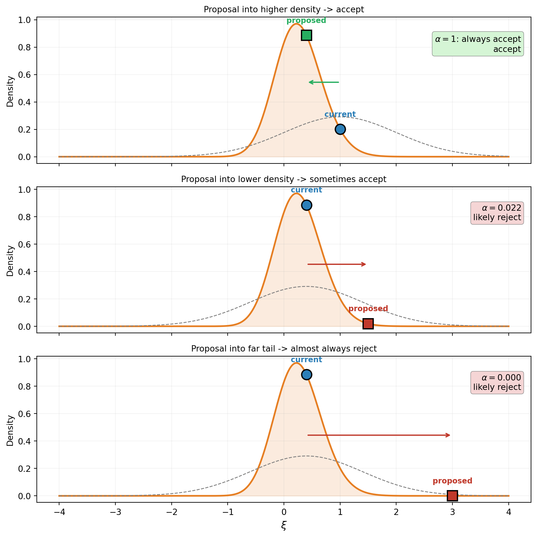
The rule in words:
- If the proposed location has higher posterior density, always accept the move.
- If the proposed location has lower posterior density, accept with probability equal to the ratio of densities: \(\alpha = p(\theta^*) / p(\theta^{(t)})\).
- If the proposed location is way out in the tail, \(\alpha \approx 0\) and the move is almost always rejected.
ImportantThe normalizing constant cancels
The acceptance ratio only needs the ratio of posterior densities: \[ \alpha = \min\!\left(1,\; \frac{p(\theta^* \mid y)}{p(\theta^{(t)} \mid y)}\right) = \min\!\left(1,\; \frac{\mathcal{L}(\theta^*)\, p(\theta^*)}{\mathcal{L}(\theta^{(t)})\, p(\theta^{(t)})}\right) \] The evidence \(p(y)\) appears in both numerator and denominator and cancels. This is why MCMC works: we never need the intractable normalizing constant.
Running MCMC on the 1D Beam
We use a cantilever beam whose bending stiffness varies spatially, parameterized by a single KLE coefficient \(\xi \sim \mathcal{N}(0, 1)\). We observe the tip deflection with 10% Gaussian noise and want to infer \(\xi\). Rather than writing a manual Metropolis-Hastings loop, we use the LogUnNormalizedPosterior and MetropolisHastingsSampler classes from the typing API.
from pyapprox.inverse.posterior.log_unnormalized import (
    LogUnNormalizedPosterior,
)
from pyapprox.inverse.sampling.metropolis import (
    MetropolisHastingsSampler,
)

# Log-posterior = log-likelihood + log-prior
posterior = LogUnNormalizedPosterior(
    model_fn=tip_model, likelihood=noise_likelihood, prior=prior, bkd=bkd,
)

# MCMC
n_steps = 2000
proposal_cov = bkd.asarray([[0.8**2]])
sampler = MetropolisHastingsSampler(
    log_posterior_fn=posterior, nvars=1, bkd=bkd, proposal_cov=proposal_cov,
)

np.random.seed(0)
result = sampler.sample(
    nsamples=n_steps, burn=0,
    initial_state=bkd.asarray([[0.0]]),  # prior mean
    bounds=bkd.asarray([[-4.0, 4.0]]),
)

chain = bkd.to_numpy(result.samples)[0, :]
print(f"Chain length: {n_steps}")
print(f"Acceptance rate: {result.acceptance_rate:.1%}")
Chain length: 2000
Acceptance rate: 51.3%Figure 3 shows the result. The trace plot (left) shows the walker bouncing around the high-density region. The histogram of chain samples (right, after discarding the first 200 steps as burn-in) closely matches the exact grid posterior.
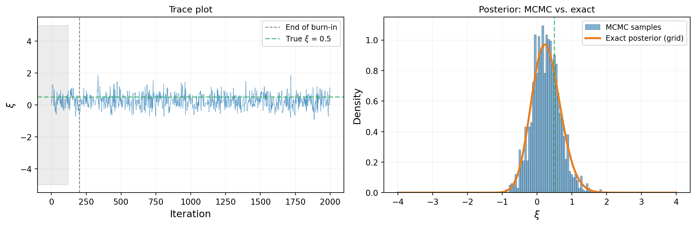
The histogram matches the exact posterior — the chain has done its job.
Extending to Two Parameters
Now consider a beam where the bending stiffness \(EI(x)\) varies along its length, parameterized by a 2-term Karhunen-Lo`eve (KLE) expansion:
\[ \log EI(x) = \log \overline{EI} + \sigma \sum_{i=1}^{2} \sqrt{\lambda_i}\, \phi_i(x)\, \xi_i \]
where \(\overline{EI}\) is the mean stiffness, \((\lambda_i, \phi_i)\) are the KLE eigenvalues and eigenfunctions, and \(\xi_1, \xi_2 \sim \mathcal{N}(0,1)\) are the uncertain parameters we want to infer. The 1D case above used a single KLE term; now we have a richer model that captures more spatial variation, making it a genuinely 2D inference problem.
# 1D FEM beam with 2 KLE terms for spatially varying EI(x)
problem_2d = build_cantilever_beam_1d(bkd, num_kle_terms=2)
beam_2d = problem_2d.function()   # nvars=2, nqoi=3
prior_2d = problem_2d.prior()     # IndependentJoint of 2 x N(0,1)

# Tip-only wrapper (first QoI is tip deflection)
tip_model_2d = FunctionFromCallable(
    nqoi=1, nvars=2,
    fun=lambda xi: beam_2d(xi)[0:1, :],
    bkd=bkd,
)

# True KLE parameters and synthetic data
xi_true_2d = bkd.asarray([[0.5], [-0.3]])
delta_true_2d = float(tip_model_2d(xi_true_2d)[0, 0])
sigma_noise_2d = 0.1 * abs(delta_true_2d)
noise_lik_2d = DiagonalGaussianLogLikelihood(
    bkd.asarray([sigma_noise_2d**2]), bkd,
)
model_lik_2d = ModelBasedLogLikelihood(tip_model_2d, noise_lik_2d, bkd)

np.random.seed(7)
y_obs_2d = float(model_lik_2d.rvs(xi_true_2d))
noise_lik_2d.set_observations(bkd.asarray([[y_obs_2d]]))

print(f"True KLE parameters:  xi = [{float(xi_true_2d[0, 0])}, "
      f"{float(xi_true_2d[1, 0])}]")
print(f"True tip deflection:  {delta_true_2d:.6f}")
print(f"Observed:             {y_obs_2d:.6f}")
print(f"Noise std (10%):      {sigma_noise_2d:.6f}")
True KLE parameters: xi = [0.5, -0.3]
True tip deflection: 8.656735
Observed: 10.120178
Noise std (10%): 0.865673# --- 2D MCMC ---
posterior_2d = LogUnNormalizedPosterior(
model_fn=tip_model_2d, likelihood=noise_lik_2d, prior=prior_2d, bkd=bkd,
)
n_steps_2d = 5000
proposal_cov_2d = bkd.asarray([[0.5**2, 0.0], [0.0, 0.5**2]])
sampler_2d = MetropolisHastingsSampler(
log_posterior_fn=posterior_2d, nvars=2, bkd=bkd,
proposal_cov=proposal_cov_2d,
)
np.random.seed(1)
result_2d = sampler_2d.sample(
nsamples=n_steps_2d, burn=0,
initial_state=bkd.asarray([[0.0], [0.0]]), # prior mean
bounds=bkd.asarray([[-4.0, 4.0], [-4.0, 4.0]]),
)
chain_2d = bkd.to_numpy(result_2d.samples).T # (n_steps, 2) for plotting
print(f"Acceptance rate: {result_2d.acceptance_rate:.1%}")Acceptance rate: 53.2%Figure 4 shows the chain exploring the 2D posterior. The trajectory starts at the prior mean (star) and migrates toward the data-consistent region, then settles into the stationary exploration pattern.
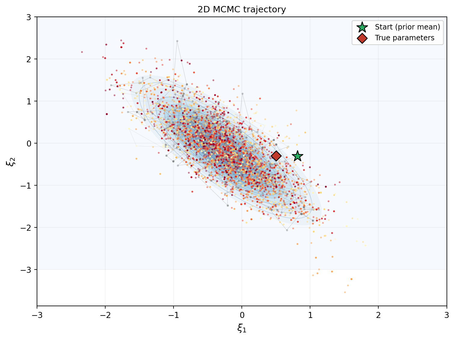
Figure 5 extracts the marginal distributions of \(\xi_1\) and \(\xi_2\) from the chain and compares them to the exact marginals from the grid posterior.

Posterior Predictive Check
As a final sanity check, we propagate every posterior sample through the model and compare the resulting distribution of predictions to the observed data. If the inference is correct, the observation should sit in the bulk of the posterior predictive distribution.
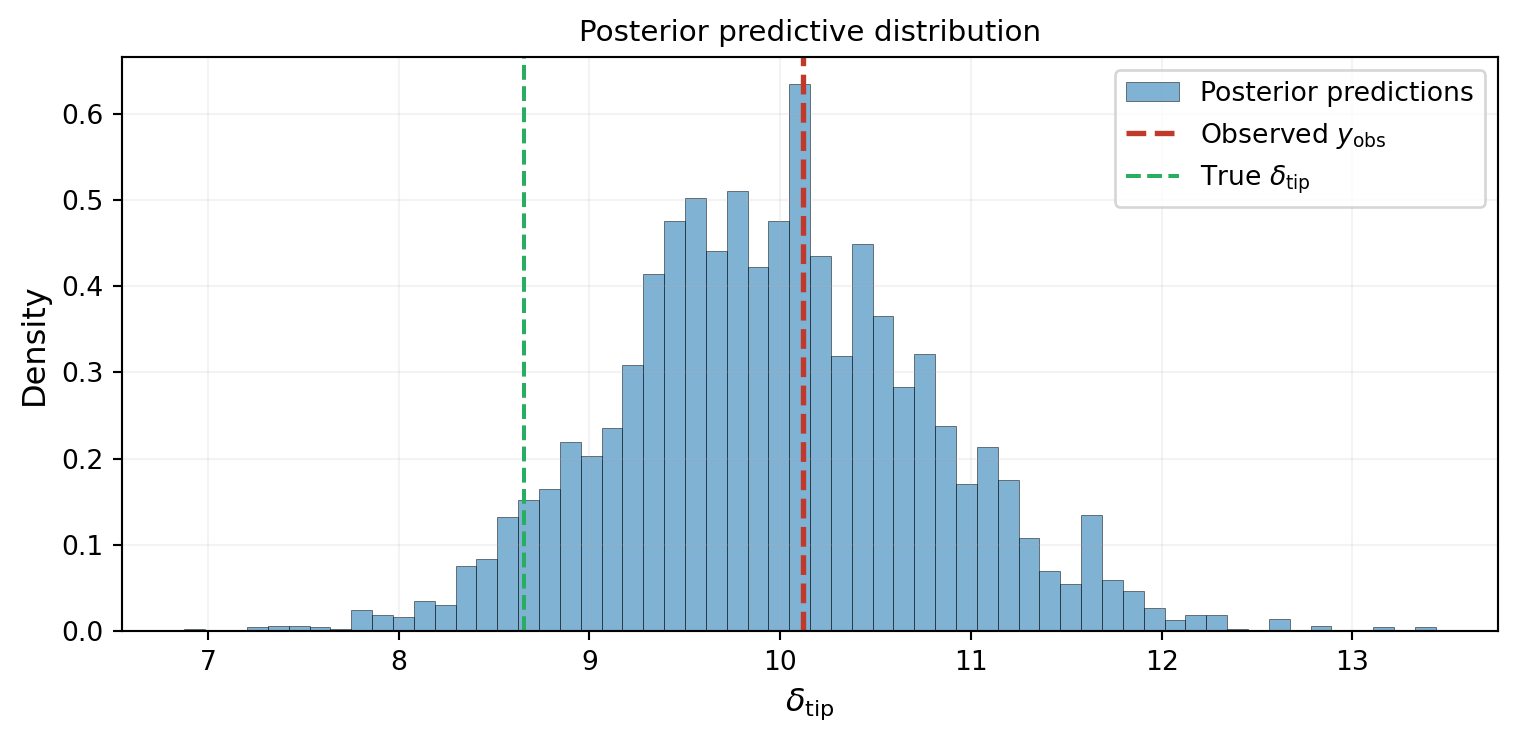
The observation sits right in the middle of the predictive distribution. The inference is working: the posterior parameters produce predictions consistent with the data.
Key Takeaways
- MCMC generates posterior samples by running a random walker that preferentially visits high-density regions
- The accept/reject mechanism uses only the ratio of posterior densities, so the normalizing constant is never needed
- The chain’s histogram converges to the posterior distribution, which we verified against the exact grid solution in both 1D and 2D
- The posterior predictive check is a simple but powerful diagnostic: if the data is inconsistent with the posterior predictions, something is wrong
- The chain’s behavior depends on choices we haven’t addressed: proposal size, burn-in length, number of steps — these are the subject of the next tutorial
Exercises
Change the starting point to \(\xi = -3\) (far from the posterior mode) in the 1D example. How many steps does the chain take to reach the high-density region? How does this affect the required burn-in?
In the 2D example, double the noise standard deviation
sigma_noise_2d. How does the posterior change? Is it wider or narrower? Does the chain need more or fewer steps to converge?Add a second observation (second measurement of tip deflection, independent noise). Create a new
DiagonalGaussianLogLikelihoodwith two noise variances and two observations, and rerun the chain. Does the posterior narrow?(Challenge) Run the 2D chain with a very large proposal covariance (e.g.,
proposal_cov_2d = bkd.asarray([[25.0, 0.0], [0.0, 25.0]])). What happens to the acceptance rate and the trace plot? Why?
Next Steps
Continue with:
- Practical MCMC: Metropolis-Hastings and DRAM — Tuning proposals, adaptive methods, and convergence diagnostics