Parametrically Defined Approximate Control Variates
PyApprox Tutorial Library
How a single integer vector — the recursion index — unifies MLMC, MFMC, ACVMF, and ACVIS as special cases of one family, and enables automatic selection of the best estimator structure for any problem.
TipDownload Notebook
Learning Objectives
After completing this tutorial, you will be able to:
- Define the recursion index \(\boldsymbol{\gamma}\) and explain how it determines which models act as control variates for which other models
- Read a recursion DAG and identify the corresponding estimator family
- Recognise MLMC, MFMC, ACVMF, and ACVIS as special cases of the PACV family
- Explain why enumerating all valid recursion indices enables automatic best-estimator selection for a given problem and budget
Prerequisites
Complete General ACV Concept before this tutorial. That tutorial establishes the CV-1 ceiling and explains why direct correction (ACVMF) beats MFMC; this tutorial generalises both into a single parametric family.
The Problem with Hand-Designed Estimators
The estimators developed so far — MLMC, MFMC, ACVMF, ACVIS — were each hand-designed for a particular belief about the model hierarchy. MLMC and MFMC assume a chain: each model corrects the one above it. ACVMF and ACVIS assume a star: every LF model corrects \(f_0\) directly. These are reasonable extremes, but neither is provably optimal for an arbitrary correlation structure.
In practice, the best correction structure for a five-model ensemble is problem-specific. Maybe \(f_1\) should directly correct \(f_0\), but \(f_2\) should correct \(f_1\), while \(f_3\) and \(f_4\) both correct \(f_0\) directly — some mixture of chain and star. There are many such structures. The question is: can they be enumerated cheaply enough to evaluate them all, and can the best one be selected from pilot data alone?
The answer is yes, via the recursion index.
The Recursion Index
A recursion index \(\boldsymbol{\gamma} = [\gamma_1, \ldots, \gamma_M]^\top\) is an integer vector, one entry per LF model. Entry \(\gamma_j = i\) means:
Model \(f_j\) acts as a control variate for model \(f_i\), i.e. \(\mathcal{Z}_j^* = \mathcal{Z}_i\).
In other words, the anchor sample set of the correction \(\Delta_j\) is the same as the full sample set of model \(f_i\).
Two constraints keep the structure well-defined:
- Valid targets: \(\gamma_j < j\) for all \(j\) (each model can only correct models with a lower index, preventing cycles).
- Zero-rooted: \(\gamma_j = 0\) means \(f_j\) directly corrects the HF model \(f_0\).
These constraints make the recursion index encode a directed acyclic graph (DAG) rooted at node 0 (the HF model), with \(M\) leaf-to-root edges.
Known Estimators as Special Cases
The recursion index recovers every estimator from previous tutorials as a single point in the parameter space:
| Estimator | Recursion index \(\boldsymbol{\gamma}\) | DAG shape |
|---|---|---|
| MLMC / MFMC | \([0, 1, 2, \ldots, M-1]\) | Chain: \(f_M \to f_{M-1} \to \cdots \to f_0\) |
| ACVMF / ACVIS | \([0, 0, 0, \ldots, 0]\) | Star: all \(f_j \to f_0\) |
| Any intermediate | \(\boldsymbol{\gamma}\) with mixed entries | Mixed tree |
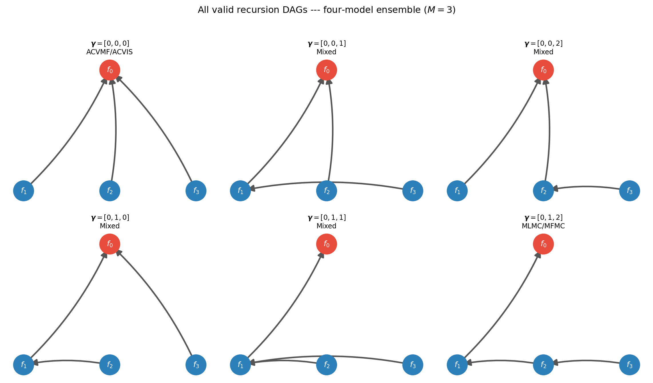
Figure 1 makes this visual for a four-model ensemble (\(M=3\), indices 1–3 for the LF models). Each subfigure is a valid recursion index; the edge from node \(j\) to node \(\gamma_j\) is drawn explicitly.
All \(3^1 \cdot 2^1 \cdot 1^1 = 6\) valid indices are shown — but wait, for \(M=3\) there are \(1 \times 2 \times 3 = 6\) valid indices (entry \(\gamma_j \in \{0, \ldots, j-1\}\), so \(j\) choices for entry \(j\), giving \(\prod_{j=1}^{M} j = M!\) total). For \(M=4\): 24 indices. For \(M=5\): 120. Still enumerable.
Three Base Families
The recursion index determines which sample sets are anchored to which, but not the detailed structure of how the anchor and exclusive partitions are arranged. That is determined by the base allocation matrix. PACV defines three families:
GMF (Generalised Multi-Fidelity): Based on the MFMC allocation matrix. If \(\gamma_j = i\), then \(\mathcal{Z}_j^* = \mathcal{Z}_i\) and \(\mathcal{Z}_i \subseteq \mathcal{Z}_j\) (the anchor set is a nested subset of the model’s full sample set). ACVMF is GMF with \(\boldsymbol{\gamma} = \mathbf{0}\); MFMC is GMF with \(\boldsymbol{\gamma} = [0,1,\ldots,M-1]\).
GRD (Generalised Recursive Difference): Based on the MLMC allocation matrix. If \(\gamma_j = i \neq j\), then \(\mathcal{Z}_i \cap \mathcal{Z}_j \neq \emptyset\) (the anchor and the model’s set overlap but neither contains the other). MLMC is GRD with \(\boldsymbol{\gamma} = [0,1,\ldots,M-1]\).
GIS (Generalised Independent Sample): Based on the ACVIS allocation matrix. If \(\gamma_j = i\), then \(\mathcal{Z}_j^* \subseteq \mathcal{Z}_j\) and the correction uses an independent sub-partition of model \(j\)’s samples as the anchor. ACVIS is GIS with \(\boldsymbol{\gamma} = \mathbf{0}\).
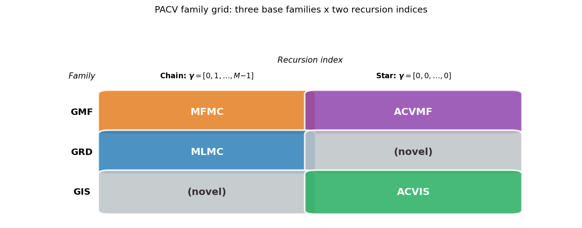
Figure 2 shows how the four classical estimators map onto this family grid.
Automatic Best-Estimator Selection
Because every valid recursion index defines a concrete estimator whose sample allocation can be optimised from the pilot covariance alone, it is possible to:
- Generate all \(M!\) recursion indices for the given number of models.
- For each index and each family (GMF, GRD, GIS), run
search.search(P). - Read off
covariance()from the best estimator. - Return the estimator with the smallest predicted variance.
This is what ACVSearch does with TreeDepthRecursionStrategy(max_depth=M-1). No model evaluations are required beyond the pilot study — selection is purely from covariance structure.

The best recursion index shifts with the cost ratio, budget, and correlation structure. Committing to MLMC or MFMC by convention can leave significant variance reduction on the table for problems where an intermediate structure is better.
Convergence to the Multi-Model CV Ceiling
Like ACVMF, the best PACV estimator converges to the multi-model CV ceiling as LF sample counts grow. Figure 4 demonstrates this by fixing the HF sample count at \(N_0 = 1\) and steadily increasing LF samples on the five-model polynomial benchmark. The best GMF curve selects the recursion index with lowest variance at each cost point (over all 125 valid indices). Both ACVMF and the best GMF converge toward the CV-4 limit, while MLMC and MFMC plateau at CV-1.

This plot mirrors the ceiling plots in the MFMC Concept and MLBLUE Concept tutorials. The best GMF envelope matches or beats ACVMF at every cost: at small budgets the best recursion index may differ from the star, while at large budgets both converge to CV-\(M\). MLMC and MFMC are permanently capped at CV-1. The key advantage of PACV is that it automatically finds the best recursion index — there is no need to guess whether the star (ACVMF) or chain (MFMC) structure is better for the problem at hand.
Key Takeaways
- The recursion index \(\boldsymbol{\gamma}\) encodes which model corrects which, as a DAG rooted at the HF model \(f_0\)
- MLMC and MFMC share the chain recursion index \([0,1,\ldots,M-1]\); ACVMF and ACVIS share the star index \([0,0,\ldots,0]\); every other valid index is a novel estimator
- Three base families (GMF, GRD, GIS) pair with the set of all recursion indices to produce the full PACV library
- For \(M\) LF models there are \(M!\) valid recursion indices — small enough to enumerate fully for typical ensemble sizes (\(M \leq 6\))
- Enumeration with
ACVSearchandTreeDepthRecursionStrategyselects the best structure from pilot data alone, without any additional model evaluations
Exercises
List all valid recursion indices for \(M = 2\) LF models. How many are there? Draw the DAG for each.
For \(M = 4\) LF models, how many valid recursion indices exist? At what \(M\) does full enumeration become computationally expensive (say, \(> 10^4\) indices)?
For the GMF family, explain in one sentence why MFMC and ACVMF are both GMF estimators but have very different variance reduction profiles.
Suppose the pilot covariance shows \(\rho_{0,2} > \rho_{0,1}\) (the second LF model is more correlated with the HF model than the first). Is the chain recursion index \(\boldsymbol{\gamma} = [0, 1]\) or \(\boldsymbol{\gamma} = [0, 0]\) more likely to be optimal? Explain using the CV ceiling argument from General ACV Concept.
Next Steps
- PACV Analysis — Formal definition of the three families, the recursive covariance formulas, and how PyApprox enumerates all valid indices
- API Cookbook — Configure, enumerate, and select the best PACV estimator for a given problem using the PyApprox API
- Ensemble Selection — Once the best structure is known, choose which subset of models to include
Tip
Ready to try this? See API Cookbook → ACVSearch.
References
[BLWLJCP2022] D. Schaden, E. Ullmann. On the optimization of approximate control variates with parametrically defined estimators. Journal of Computational Physics, 451:110882, 2022. DOI
[GGEJJCP2020] A. Gorodetsky, S. Geraci, M. Eldred, J. Jakeman. A generalized approximate control variate framework for multifidelity uncertainty quantification. Journal of Computational Physics, 408:109257, 2020. DOI