Let \(f_0, \ldots, f_M\) be a model hierarchy with per-sample costs \(C_0 > \cdots > C_M\). Write \(\rho_\alpha = \rho_{0,\alpha}\) for the correlation between \(f_\alpha\) and the HF model (\(\rho_0 = 1\), \(\rho_{M+1} = 0\) by convention). Let \(N_\alpha = r_\alpha N_0\) be the total number of samples evaluated by model \(\alpha\), with \(r_0 = 1\) and \(r_1 \leq r_2 \leq \cdots \leq r_M\) (nested).
so that \(\mathcal{Z}_\alpha = p_0 \cup p_1 \cup \cdots \cup p_\alpha\). Partition \(p_\alpha\) has \(N_\alpha - N_{\alpha-1} = (r_\alpha - r_{\alpha-1})N_0\) samples and is independent of all other partitions. The total cost is
Using the partition decomposition, we can write \(\hat{\mu}_\alpha(\mathcal{Z}_\alpha) = \frac{N_{\alpha-1}}{N_\alpha}\hat{\mu}_\alpha(\mathcal{Z}_{\alpha-1}) + \frac{|p_\alpha|}{N_\alpha}\hat{\mu}_\alpha(p_\alpha)\), so
This mirrors the two-model ACV correction variance from ACV Analysis, with the pair \((r_{\alpha-1},\, r_\alpha)\) playing the roles of \((1,\, r)\).
Covariance Between HF Estimator and Each Correction
Since \(\mathcal{Z}_0 \subset \mathcal{Z}_{\alpha-1}\), the HF mean \(\hat{\mu}_0(\mathcal{Z}_0)\) shares all \(N_0\) samples with \(\hat{\mu}_\alpha(\mathcal{Z}_{\alpha-1})\) but shares none with \(\hat{\mu}_\alpha(p_\alpha)\). Therefore
Note this has the same \((r_{\alpha-1}^{-1} - r_\alpha^{-1})\) factor as the correction variance Equation 3, which will produce a clean cancellation when we optimise \(\eta_\alpha\).
Optimal Weights and Variance Reduction
Corrections at different levels use different independent exclusive partitions, so \(\mathrm{Cov}(\Delta_\alpha, \Delta_\beta) = 0\) for \(\alpha \neq \beta\) (both corrections use the shared \(\mathcal{Z}_0\) samples, but after the optimal weight minimisation these cross-terms vanish from the variance expression). The full variance is
The variance reduction relative to MC is \(1 - \sum_\alpha (r_{\alpha-1}^{-1} - r_\alpha^{-1})\rho_\alpha^2\). As \(r_\alpha \to \infty\) for all \(\alpha\), this approaches \(1 - \rho_1^2\), the CV-1 limit identified in the concept tutorial.
Optimal Sample Ratios
Minimise Equation 6 subject to the cost constraint Equation 1. Both variance and cost depend on \(N_0\) and \(r_1, \ldots, r_M\). Treating these as continuous variables and differentiating with respect to \(r_\alpha\) yields the optimal ratios [PWGSIAM2016]:
The factor \(\rho_\alpha^2 - \rho_{\alpha+1}^2\) is the marginal correlation gain from adding model \(\alpha\): how much additional correlation with \(f_0\) model \(\alpha\) provides over the next cheaper model. A large marginal gain and low cost \(C_\alpha\) together produce a large \(r_\alpha^*\) — many samples are worth allocating to that level.
ImportantValidity condition
The formula Equation 7 requires the ratios to be strictly increasing (\(r_\alpha^* > r_{\alpha-1}^*\)). This holds when
Interpretation: The cost ratio between adjacent models must exceed the ratio of their marginal correlation gains. If this fails for model \(\alpha\), that model does not contribute to variance reduction at the optimal allocation and should be removed from the hierarchy before solving again.
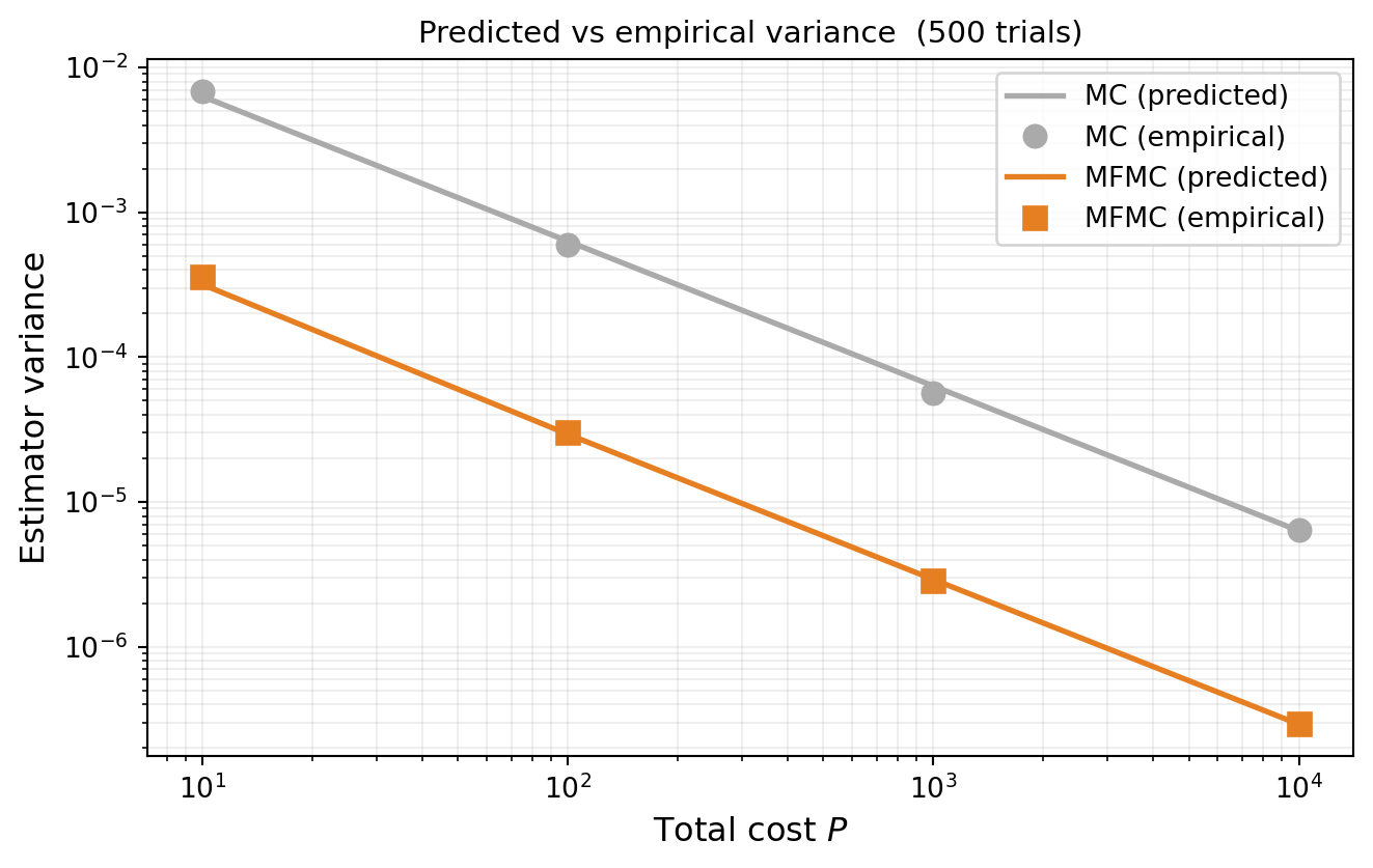
Figure 1: MFMC and MC variance vs total cost: covariance() predictions (lines) compared to empirical variance from 500 independent trials (markers). Close agreement confirms the estimator’s variance prediction is accurate.
Key Takeaways
The partition decomposition makes the variance calculation clean: \(\mathbb{V}[\Delta_\alpha] = \frac{\sigma_\alpha^2}{N_0}(r_{\alpha-1}^{-1} - r_\alpha^{-1})\) and \(\mathrm{Cov}(\hat{\mu}_0, \Delta_\alpha) = \frac{C_{0\alpha}}{N_0}(r_{\alpha-1}^{-1} - r_\alpha^{-1})\)
The optimal weight \(\eta_\alpha^* = -\rho_\alpha \sigma_0 / \sigma_\alpha\) is the same at every level and matches the two-model ACV formula
The MFMC variance reduction is \(1 - \sum_\alpha (r_{\alpha-1}^{-1} - r_\alpha^{-1})\rho_\alpha^2\), converging to \(1 - \rho_1^2\) as all ratios grow
The optimal ratio \(r_\alpha^* \propto \sqrt{(\rho_\alpha^2 - \rho_{\alpha+1}^2)/C_\alpha}\) is large when model \(\alpha\) is cheap and has a large marginal correlation gain
The validity condition must hold for every model; violators should be dropped from the hierarchy
Exercises
For \(M = 1\), verify that Equation 7 reduces to the two-model ACV optimal ratio \(r^* = \sqrt{C_0\rho_1^2 / (C_1(1-\rho_1^2))}\) from ACV Analysis.
Show algebraically that as \(r_\alpha \to \infty\) for all \(\alpha\), the variance Equation 6 approaches \(\sigma_0^2(1-\rho_1^2)/N_0\) (the CV-1 limit).
For the polynomial benchmark, compute the MFMC minimum cost to achieve \(\epsilon^2 = 10^{-4}\) and compare it to the MLMC minimum cost from MLMC Analysis. Which is smaller?
(Challenge) Verify the claim that corrections at different levels satisfy \(\mathrm{Cov}(\Delta_\alpha, \Delta_\beta) = 0\) for the specific case \(\alpha=1\), \(\beta=2\) by writing each \(\Delta\) in terms of independent partition means and expanding the covariance directly.
References
[PWGSIAM2016] B. Peherstorfer, K. Willcox, M. Gunzburger. Optimal Model Management for Multifidelity Monte Carlo Estimation. SIAM Journal on Scientific Computing, 38(5):A3163–A3194, 2016. DOI
[GGLZ2022] A. Gruber, M. Gunzburger, L. Ju et al. A Multifidelity Monte Carlo Method for Realistic Computational Budgets. Journal of Scientific Computing, 94:2, 2023. DOI
Source Code
---title: "Multi-Fidelity Monte Carlo: Analysis"subtitle: "PyApprox Tutorial Library"description: "Deriving the MFMC estimator variance from its partition structure, the optimal weights and sample ratios, and the validity condition."tutorial_type: analysistopic: multi_fidelitydifficulty: intermediateestimated_time: 15render_time: 50prerequisites: - mfmc_concept - mlmc_analysistags: - multi-fidelity - mfmc - optimal-allocation - estimator-theoryformat: html: code-fold: false code-tools: true toc: true fig-dpi: 96execute: echo: true warning: falsejupyter: python3---::: {.callout-tip collapse="true"}## Download Notebook[Download as Jupyter Notebook](notebooks/mfmc_analysis.ipynb):::## Learning ObjectivesAfter completing this tutorial, you will be able to:- Decompose the MFMC sample structure into independent partitions and use this to derive the variance of each correction term- Derive the optimal weights $\eta_\alpha^*$ and the resulting variance formula- Derive the optimal sample ratios $r_\alpha^*$ and state the validity condition- Verify the API's predicted variance against empirical trials## PrerequisitesComplete [MFMC Concept](mfmc_concept.qmd) and [MLMC Analysis](mlmc_analysis.qmd)before this tutorial.## Setup and NotationLet $f_0, \ldots, f_M$ be a model hierarchy with per-sample costs $C_0 > \cdots > C_M$.Write $\rho_\alpha = \rho_{0,\alpha}$ for the correlation between $f_\alpha$ and the HFmodel ($\rho_0 = 1$, $\rho_{M+1} = 0$ by convention). Let $N_\alpha = r_\alpha N_0$be the total number of samples evaluated by model $\alpha$, with $r_0 = 1$ and$r_1 \leq r_2 \leq \cdots \leq r_M$ (nested).Define the **independent sample partitions**$$p_0 = \mathcal{Z}_0,\qquadp_\alpha = \mathcal{Z}_\alpha \setminus \mathcal{Z}_{\alpha-1},\quad \alpha = 1,\ldots,M,$$so that $\mathcal{Z}_\alpha = p_0 \cup p_1 \cup \cdots \cup p_\alpha$. Partition $p_\alpha$has $N_\alpha - N_{\alpha-1} = (r_\alpha - r_{\alpha-1})N_0$ samples and is independent ofall other partitions. The total cost is$$C_{\text{tot}} = \sum_{\alpha=0}^M |p_\alpha| C_\alpha= N_0 \sum_{\alpha=0}^M (r_\alpha - r_{\alpha-1}) C_\alpha.$$ {#eq-cost}The MFMC estimator is$$\hat{\mu}_0^{\text{MFMC}} = \hat{\mu}_0(\mathcal{Z}_0)+ \sum_{\alpha=1}^{M} \eta_\alpha \underbrace{\bigl(\hat{\mu}_\alpha(\mathcal{Z}_{\alpha-1}) - \hat{\mu}_\alpha(\mathcal{Z}_\alpha)\bigr)}_{\Delta_\alpha}.$$ {#eq-mfmc}## Variance of Each Correction TermUsing the partition decomposition, we can write$\hat{\mu}_\alpha(\mathcal{Z}_\alpha) = \frac{N_{\alpha-1}}{N_\alpha}\hat{\mu}_\alpha(\mathcal{Z}_{\alpha-1}) + \frac{|p_\alpha|}{N_\alpha}\hat{\mu}_\alpha(p_\alpha)$, so$$\Delta_\alpha= \hat{\mu}_\alpha(\mathcal{Z}_{\alpha-1}) - \hat{\mu}_\alpha(\mathcal{Z}_\alpha)= \frac{|p_\alpha|}{N_\alpha} \Bigl(\hat{\mu}_\alpha(\mathcal{Z}_{\alpha-1}) - \hat{\mu}_\alpha(p_\alpha)\Bigr).$$Since $\mathcal{Z}_{\alpha-1}$ and $p_\alpha$ are independent,$$\mathbb{V}[\Delta_\alpha]= \frac{|p_\alpha|^2}{N_\alpha^2} \left(\frac{\sigma_\alpha^2}{N_{\alpha-1}} + \frac{\sigma_\alpha^2}{|p_\alpha|}\right)= \frac{\sigma_\alpha^2 |p_\alpha|}{N_\alpha^2} \left(\frac{|p_\alpha|}{N_{\alpha-1}} + 1\right).$$Substituting $N_\alpha = r_\alpha N_0$, $N_{\alpha-1} = r_{\alpha-1} N_0$,$|p_\alpha| = (r_\alpha - r_{\alpha-1})N_0$:$$\mathbb{V}[\Delta_\alpha]= \frac{\sigma_\alpha^2}{N_0} \left(\frac{1}{r_{\alpha-1}} - \frac{1}{r_\alpha}\right).$$ {#eq-delta-var}This mirrors the two-model ACV correction variance from [ACV Analysis](acv_many_models_analysis.qmd#sec-two-model),with the pair $(r_{\alpha-1},\, r_\alpha)$ playing the roles of $(1,\, r)$.## Covariance Between HF Estimator and Each CorrectionSince $\mathcal{Z}_0 \subset \mathcal{Z}_{\alpha-1}$, the HF mean $\hat{\mu}_0(\mathcal{Z}_0)$shares all $N_0$ samples with $\hat{\mu}_\alpha(\mathcal{Z}_{\alpha-1})$ but shares nonewith $\hat{\mu}_\alpha(p_\alpha)$. Therefore$$\mathrm{Cov}\bigl(\hat{\mu}_0(\mathcal{Z}_0),\; \Delta_\alpha\bigr)= \mathrm{Cov}\!\left(\hat{\mu}_0(\mathcal{Z}_0),\; \hat{\mu}_\alpha(\mathcal{Z}_{\alpha-1})\right)- \underbrace{\mathrm{Cov}\!\left(\hat{\mu}_0(\mathcal{Z}_0),\; \hat{\mu}_\alpha(p_\alpha)\right)}_{=\,0}.$$The first term has $N_0$ shared samples out of $N_{\alpha-1}$:$$\mathrm{Cov}\bigl(\hat{\mu}_0(\mathcal{Z}_0),\; \hat{\mu}_\alpha(\mathcal{Z}_{\alpha-1})\bigr)= \frac{N_0}{N_0 N_{\alpha-1}}\,C_{0\alpha}= \frac{C_{0\alpha}}{r_{\alpha-1} N_0},$$where $C_{0\alpha} = \mathrm{Cov}(f_0, f_\alpha)$. Hence$$\mathrm{Cov}\bigl(\hat{\mu}_0(\mathcal{Z}_0),\; \Delta_\alpha\bigr)= \frac{C_{0\alpha}}{N_0}\left(\frac{1}{r_{\alpha-1}} - \frac{1}{r_\alpha}\right).$$ {#eq-cross-cov}Note this has the same $(r_{\alpha-1}^{-1} - r_\alpha^{-1})$ factor as the correctionvariance @eq-delta-var, which will produce a clean cancellation when we optimise $\eta_\alpha$.## Optimal Weights and Variance ReductionCorrections at different levels use different independent exclusive partitions, so$\mathrm{Cov}(\Delta_\alpha, \Delta_\beta) = 0$ for $\alpha \neq \beta$ (both correctionsuse the shared $\mathcal{Z}_0$ samples, but after the optimal weight minimisation thesecross-terms vanish from the variance expression). The full variance is$$\mathbb{V}[\hat{\mu}_0^{\text{MFMC}}]= \frac{\sigma_0^2}{N_0}+ \sum_{\alpha=1}^M \eta_\alpha^2\, \mathbb{V}[\Delta_\alpha]+ 2\sum_{\alpha=1}^M \eta_\alpha\, \mathrm{Cov}\bigl(\hat{\mu}_0,\, \Delta_\alpha\bigr).$$Substituting @eq-delta-var and @eq-cross-cov and minimising over $\eta_\alpha$(each term is independent, so we minimise each separately):$$\eta_\alpha^* = -\frac{\mathrm{Cov}(\hat{\mu}_0,\, \Delta_\alpha)}{\mathbb{V}[\Delta_\alpha]}= -\frac{C_{0\alpha}}{\sigma_\alpha^2}= -\frac{\rho_\alpha \sigma_0}{\sigma_\alpha}.$$ {#eq-eta-star}Substituting $\eta_\alpha^*$ back and using $C_{0\alpha} = \rho_\alpha \sigma_0 \sigma_\alpha$:$$\boxed{\mathbb{V}[\hat{\mu}_0^{\text{MFMC}}]= \frac{\sigma_0^2}{N_0} \left(1 - \sum_{\alpha=1}^{M} \left(\frac{1}{r_{\alpha-1}} - \frac{1}{r_\alpha}\right)\rho_\alpha^2 \right).}$$ {#eq-mfmc-var}The variance reduction relative to MC is $1 - \sum_\alpha (r_{\alpha-1}^{-1} - r_\alpha^{-1})\rho_\alpha^2$.As $r_\alpha \to \infty$ for all $\alpha$, this approaches $1 - \rho_1^2$, the CV-1 limitidentified in the concept tutorial.## Optimal Sample RatiosMinimise @eq-mfmc-var subject to the cost constraint @eq-cost. Both variance and costdepend on $N_0$ and $r_1, \ldots, r_M$. Treating these as continuous variables anddifferentiating with respect to $r_\alpha$ yields the optimal ratios [PWGSIAM2016]:$$\boxed{r_\alpha^* = \sqrt{ \frac{C_0\,(\rho_\alpha^2 - \rho_{\alpha+1}^2)} {C_\alpha\,(1 - \rho_1^2)}},\quad \alpha = 1, \ldots, M.}$$ {#eq-r-star}The factor $\rho_\alpha^2 - \rho_{\alpha+1}^2$ is the marginal correlation gain fromadding model $\alpha$: how much additional correlation with $f_0$ model $\alpha$ providesover the next cheaper model. A large marginal gain and low cost $C_\alpha$ together producea large $r_\alpha^*$ — many samples are worth allocating to that level.::: {.callout-important}## Validity conditionThe formula @eq-r-star requires the ratios to be strictly increasing($r_\alpha^* > r_{\alpha-1}^*$). This holds when$$\frac{C_{\alpha-1}}{C_\alpha}> \frac{\rho_{\alpha-1}^2 - \rho_\alpha^2}{\rho_\alpha^2 - \rho_{\alpha+1}^2},\quad \alpha = 1, \ldots, M.$$ {#eq-validity}**Interpretation:** The cost ratio between adjacent models must exceed the ratio of theirmarginal correlation gains. If this fails for model $\alpha$, that model does notcontribute to variance reduction at the optimal allocation and should be removed from thehierarchy before solving again.:::## Numerical Verification```{python}import numpy as npimport matplotlib.pyplot as pltfrom pyapprox.util.backends.numpy import NumpyBkdfrom pyapprox_benchmarks.statest import ( PolynomialEnsembleBenchmark,)from pyapprox.statest.statistics import MultiOutputMeanfrom pyapprox.statest.acv import MFMCEstimator, MLMCEstimatorfrom pyapprox.statest.acv.allocation import default_allocator_factoryfrom pyapprox.statest.acv.base import FittedACVEstimatorfrom pyapprox.statest.mc_estimator import MCEstimatorfrom pyapprox.statest.allocation import MCAllocatorbkd = NumpyBkd()benchmark = PolynomialEnsembleBenchmark(bkd, nmodels=5)variable = benchmark.problem().prior()models = benchmark.problem().models()costs_bkd = benchmark.problem().costs()costs = bkd.to_numpy(costs_bkd)nqoi = models[0].nqoi()cov_true = bkd.to_numpy(benchmark.ensemble_covariance())sigma2_hf = cov_true[0, 0]M =len(models) -1# Correlations rho_{0,alpha}rho = np.array([cov_true[0, a] / np.sqrt(cov_true[0, 0] * cov_true[a, a])for a inrange(len(models))])rho_ext = np.append(rho, 0.0) # rho_{M+1} = 0# Analytical optimal ratios from eq-r-starr_star = np.array([1.0] + [ np.sqrt(costs[0] * (rho_ext[a]**2- rho_ext[a+1]**2)/ (costs[a] * (1- rho_ext[1]**2)))for a inrange(1, M +1)])print("Optimal ratios r_alpha*:")for a, r inenumerate(r_star):print(f" alpha={a}: r* = {r:.2f}")``````{python}#| fig-cap: "MFMC and MC variance vs total cost: `covariance()` predictions (lines) compared to empirical variance from 500 independent trials (markers). Close agreement confirms the estimator's variance prediction is accurate."#| label: fig-variance-verifyfrom pyapprox_tutorials.figures._hierarchy import plot_mfmc_variance_verifystat = MultiOutputMean(nqoi, bkd)stat.set_pilot_quantities(bkd.asarray(cov_true))stat_mc = MultiOutputMean(nqoi, bkd)stat_mc.set_pilot_quantities(bkd.asarray(cov_true[:1, :1]))target_costs_sweep = [10, 100, 1000, 10000]n_trials =500mfmc_vars_pred, mc_vars_pred = [], []mfmc_vars_emp, mc_vars_emp = [], []for P_t in target_costs_sweep:# --- Predicted variance from fitted estimator covariance --- mf_e = MFMCEstimator(stat, costs_bkd) mf_fitted = FittedACVEstimator( mf_e, default_allocator_factory(mf_e).allocate(float(P_t)) ) mfmc_vars_pred.append(float(mf_fitted.covariance()[0, 0])) mc_e = MCEstimator(stat_mc, costs=[costs_bkd[0]]) mc_fitted = MCAllocator(mc_e).allocate(float(P_t)) mc_vars_pred.append(float(mc_fitted.covariance()[0, 0]))# --- Empirical variance from trials --- mc_ests_t = np.empty(n_trials) mfmc_ests_t = np.empty(n_trials)for i inrange(n_trials): np.random.seed(i +int(P_t) *100) [s_mc] = mc_fitted.generate_samples_per_model(variable.rvs) mc_ests_t[i] = bkd.to_numpy(mc_fitted(models[0](s_mc)))[0] s_per_m = mf_fitted.generate_samples_per_model(variable.rvs) v_per_m = [models[a](s_per_m[a]) for a inrange(len(models))] mfmc_ests_t[i] =float(mf_fitted(v_per_m)) mc_vars_emp.append(mc_ests_t.var()) mfmc_vars_emp.append(mfmc_ests_t.var())fig, ax = plt.subplots(figsize=(7, 4.5))plot_mfmc_variance_verify(target_costs_sweep, mc_vars_pred, mc_vars_emp, mfmc_vars_pred, mfmc_vars_emp, n_trials, ax)plt.tight_layout()plt.show()```## Key Takeaways- The partition decomposition makes the variance calculation clean: $\mathbb{V}[\Delta_\alpha] = \frac{\sigma_\alpha^2}{N_0}(r_{\alpha-1}^{-1} - r_\alpha^{-1})$ and $\mathrm{Cov}(\hat{\mu}_0, \Delta_\alpha) = \frac{C_{0\alpha}}{N_0}(r_{\alpha-1}^{-1} - r_\alpha^{-1})$- The optimal weight $\eta_\alpha^* = -\rho_\alpha \sigma_0 / \sigma_\alpha$ is the same at every level and matches the two-model ACV formula- The MFMC variance reduction is $1 - \sum_\alpha (r_{\alpha-1}^{-1} - r_\alpha^{-1})\rho_\alpha^2$, converging to $1 - \rho_1^2$ as all ratios grow- The optimal ratio $r_\alpha^* \propto \sqrt{(\rho_\alpha^2 - \rho_{\alpha+1}^2)/C_\alpha}$ is large when model $\alpha$ is cheap and has a large marginal correlation gain- The validity condition must hold for every model; violators should be dropped from the hierarchy## Exercises1. For $M = 1$, verify that @eq-r-star reduces to the two-model ACV optimal ratio $r^* = \sqrt{C_0\rho_1^2 / (C_1(1-\rho_1^2))}$ from [ACV Analysis](acv_many_models_analysis.qmd#sec-two-model).2. Show algebraically that as $r_\alpha \to \infty$ for all $\alpha$, the variance @eq-mfmc-var approaches $\sigma_0^2(1-\rho_1^2)/N_0$ (the CV-1 limit).3. For the polynomial benchmark, compute the MFMC minimum cost to achieve $\epsilon^2 = 10^{-4}$ and compare it to the MLMC minimum cost from[MLMC Analysis](mlmc_analysis.qmd). Which is smaller?4. **(Challenge)** Verify the claim that corrections at different levels satisfy $\mathrm{Cov}(\Delta_\alpha, \Delta_\beta) = 0$ for the specific case $\alpha=1$, $\beta=2$ by writing each $\Delta$ in terms of independent partition means and expanding the covariance directly.## References- [PWGSIAM2016] B. Peherstorfer, K. Willcox, M. Gunzburger. *Optimal Model Management for Multifidelity Monte Carlo Estimation.* SIAM Journal on Scientific Computing, 38(5):A3163--A3194, 2016. [DOI](https://doi.org/10.1137/15M1046472)- [GGLZ2022] A. Gruber, M. Gunzburger, L. Ju et al. *A Multifidelity Monte Carlo Method for Realistic Computational Budgets.* Journal of Scientific Computing, 94:2, 2023.[DOI](https://doi.org/10.1007/s10915-022-02051-y)