---
title: "Multi-Level Monte Carlo: Analysis"
subtitle: "PyApprox Tutorial Library"
description: "Deriving the optimal MLMC sample allocation, minimum achievable cost, and the MLMC complexity theorem."
tutorial_type: analysis
topic: multi_fidelity
difficulty: intermediate
estimated_time: 20
render_time: 76
prerequisites:
- mlmc_concept
- acv_many_models_analysis
tags:
- multi-fidelity
- multi-level
- optimal-allocation
- complexity-theorem
- estimator-theory
format:
html:
code-fold: false
code-tools: true
toc: true
execute:
echo: true
warning: false
jupyter: python3
---
::: {.callout-tip collapse="true"}
## Download Notebook
[Download as Jupyter Notebook](notebooks/mlmc_analysis.ipynb)
:::
## Learning Objectives
After completing this tutorial, you will be able to:
- Derive the optimal MLMC sample allocation $N_\ell^*$ via Lagrange multipliers
- State the minimum cost needed to achieve a target estimator variance $\epsilon^2$
- Verify the optimal allocation and variance reduction numerically
- Explain the connection between MLMC and ACV and when $\eta = -1$ is suboptimal
## Prerequisites
Complete [MLMC Concept](mlmc_concept.qmd) and [ACV Analysis](acv_many_models_analysis.qmd#sec-two-model) before
this tutorial.
## Setup and Notation
Let $f_0, \ldots, f_M$ be a model hierarchy ordered by decreasing fidelity, with
$f_{M+1} \equiv 0$. Define level corrections
$$
Y_\ell = f_\ell - f_{\ell+1}, \quad \ell = 0, \ldots, M.
$$
Write $V_\ell = \mathbb{V}[Y_\ell]$ and $C_\ell$ for the per-sample cost of evaluating
$f_\ell$ (note each $Y_\ell$ evaluation costs $C_\ell + C_{\ell+1}$; for brevity we absorb
this into a single level cost). Let $N_\ell = |\mathcal{Z}_\ell|$ be the number of
independent samples allocated to level $\ell$.
The MLMC estimator and its variance are
$$
\hat{\mu}_0^{\text{ML}} = \sum_{\ell=0}^{M} \hat{Y}_\ell, \qquad
\mathbb{V}[\hat{\mu}_0^{\text{ML}}] = \sum_{\ell=0}^{M} \frac{V_\ell}{N_\ell}.
$$ {#eq-mlmc-var}
The total cost is
$$
C_{\text{tot}} = \sum_{\ell=0}^{M} N_\ell C_\ell.
$$ {#eq-cost}
## Optimal Sample Allocation
We seek the $N_0, \ldots, N_M$ that minimise total cost $C_{\text{tot}}$ subject to
the variance constraint $\mathbb{V}[\hat{\mu}_0^{\text{ML}}] = \epsilon^2$.
Form the Lagrangian with multiplier $\lambda^2$:
$$
\mathcal{J} = \sum_{\ell=0}^{M} N_\ell C_\ell
+ \lambda^2 \left(\sum_{\ell=0}^{M} \frac{V_\ell}{N_\ell} - \epsilon^2\right).
$$
Setting $\partial \mathcal{J} / \partial N_\ell = 0$:
$$
C_\ell - \lambda^2 \frac{V_\ell}{N_\ell^2} = 0
\implies
\boxed{N_\ell^* = \lambda \sqrt{\frac{V_\ell}{C_\ell}}}.
$$ {#eq-optimal-N}
The optimal allocation assigns more samples to levels with **high correction variance**
and **low cost**. High-fidelity levels (small $\ell$) have large $V_\ell$ but also large
$C_\ell$; cheap levels have small $V_\ell$ but also small $C_\ell$. The ratio
$\sqrt{V_\ell / C_\ell}$ balances these competing effects.
## Minimum Cost for Target Variance
To find $\lambda$, substitute @eq-optimal-N into the variance constraint:
$$
\sum_{\ell=0}^{M} \frac{V_\ell}{N_\ell^*}
= \sum_{\ell=0}^{M} \frac{V_\ell}{\lambda\sqrt{V_\ell / C_\ell}}
= \frac{1}{\lambda} \sum_{\ell=0}^{M} \sqrt{V_\ell C_\ell} = \epsilon^2
\implies \lambda = \frac{1}{\epsilon^2} \sum_{\ell=0}^{M} \sqrt{V_\ell C_\ell}.
$$
Substituting back into @eq-cost:
$$
C_{\text{tot}}^* = \sum_{\ell=0}^{M} N_\ell^* C_\ell
= \lambda \sum_{\ell=0}^{M} \sqrt{V_\ell C_\ell}
= \frac{1}{\epsilon^2} \left(\sum_{\ell=0}^{M} \sqrt{V_\ell C_\ell}\right)^2.
$$ {#eq-min-cost}
This is the central result of MLMC. The minimum cost to achieve variance $\epsilon^2$ scales
as $\epsilon^{-2}$ (the same dimension-independent rate as plain MC), but the constant
$\left(\sum_\ell \sqrt{V_\ell C_\ell}\right)^2$ can be dramatically smaller than the MC
constant $\sigma^2_0 / C_0$ whenever the level corrections are cheap to estimate.
::: {.callout-note}
## Comparing to single-level MC
Plain MC achieves $\mathbb{V}[\hat{\mu}_0] = \sigma^2_0 / N$ at cost $N C_0$, giving
minimum cost $C_0 \sigma^2_0 / \epsilon^2$. The MLMC improvement factor is
$$
\frac{C_{\text{tot}}^*}{C_{\text{MC}}^*}
= \frac{\left(\sum_\ell \sqrt{V_\ell C_\ell}\right)^2}{C_0 \sigma^2_0}.
$$
This ratio is less than 1 (MLMC wins) whenever the hierarchy concentrates inexpensive
correction variance at cheaper levels faster than the cost per sample decreases.
:::
## Complexity Theorem
When the level corrections arise from mesh refinement at rate $h_\ell \propto 2^{-\ell}$
and satisfy standard regularity assumptions, the following decay rates hold:
$$
V_\ell \leq C_V \cdot 2^{-\alpha \ell}, \qquad C_\ell \leq C_C \cdot 2^{\beta \ell},
$$
where $\alpha > 0$ is the rate of variance decay and $\beta > 0$ is the rate of cost
growth. Under these conditions, @eq-min-cost gives the complexity theorem [GAN2015]:
$$
C_{\text{tot}}^* = \mathcal{O}\!\left(\epsilon^{-2}\right), \quad \alpha > \beta/2.
$$
When $\alpha \leq \beta/2$ the cost grows faster than $\epsilon^{-2}$, but MLMC still
outperforms plain MC by a logarithmic factor. The key message is that **if the variance
of level corrections decays faster than cost grows, MLMC achieves the same asymptotic
rate as MC but with a far smaller constant.**
## Numerical Verification
We verify @eq-optimal-N and @eq-min-cost on the five-level polynomial benchmark
$f_\ell(z) = z^{5-\ell}$, $z \sim \mathcal{U}[0,1]$, where the true $V_\ell$ can be
computed exactly.
```{python}
import numpy as np
import matplotlib.pyplot as plt
from pyapprox.util.backends.numpy import NumpyBkd
from pyapprox_benchmarks.statest import (
    PolynomialEnsembleBenchmark,
)
from pyapprox.statest.statistics import MultiOutputMean
from pyapprox.statest import MLMCEstimator
from pyapprox.statest.mc_estimator import MCEstimator
from pyapprox.statest.acv.allocation import default_allocator_factory
from pyapprox.statest.acv.base import FittedACVEstimator
from pyapprox.statest.allocation import MCAllocator

bkd = NumpyBkd()
benchmark = PolynomialEnsembleBenchmark(bkd, nmodels=5)
variable  = benchmark.problem().prior()
models    = benchmark.problem().models()
costs     = bkd.to_numpy(benchmark.problem().costs())
nqoi      = models[0].nqoi()
M         = len(models) - 1

# Exact covariance from benchmark
cov_true = bkd.to_numpy(benchmark.ensemble_covariance())
sigma2_hf = cov_true[0, 0]

# --- MLMC via estimator ---
P = 100.0
stat = MultiOutputMean(nqoi, bkd)
stat.set_pilot_quantities(bkd.asarray(cov_true))

mlmc_est = MLMCEstimator(stat, bkd.asarray(costs))
mlmc_fitted = FittedACVEstimator(
    mlmc_est, default_allocator_factory(mlmc_est).allocate(P))
N_est = bkd.to_numpy(mlmc_fitted.nsamples_per_model())
var_est = float(mlmc_fitted.covariance()[0, 0])

# --- MC via estimator ---
stat_mc = MultiOutputMean(nqoi, bkd)
stat_mc.set_pilot_quantities(bkd.asarray(cov_true[0:1, 0:1]))
mc_est = MCEstimator(stat_mc, bkd.asarray(costs[0:1]))
mc_fitted = MCAllocator(mc_est).allocate(P)
var_mc = float(mc_fitted.covariance()[0, 0])

print(f"MLMC optimized variance: {var_est:.6f}")
print(f"MC variance:            {var_mc:.6f}")
print(f"Variance reduction:     {var_mc / var_est:.1f}x")
```
```{python}
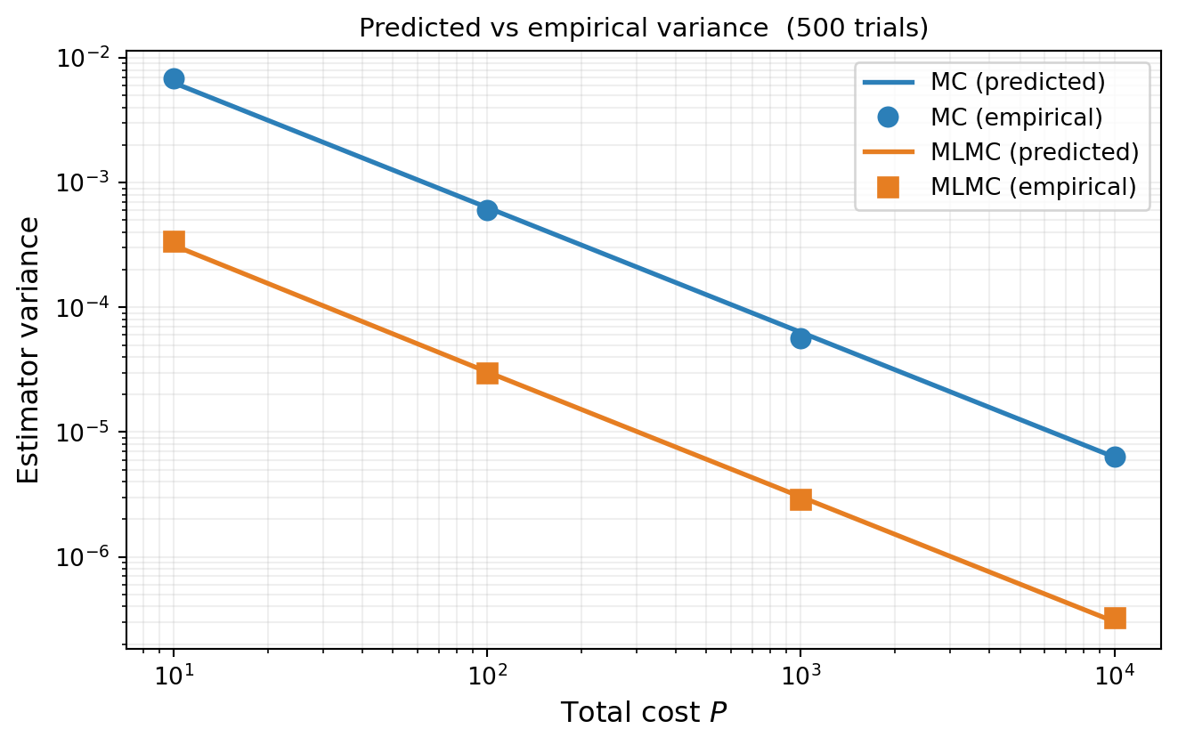
#| fig-cap: "MLMC variance vs total cost: `covariance()` (lines) compared to empirical variance from 500 independent trials (markers). Both MC (blue) and MLMC (orange) show close agreement, confirming the estimator's variance prediction. The vertical gap is the MLMC improvement factor."
#| label: fig-variance-vs-cost
from pyapprox_tutorials.figures._hierarchy import plot_variance_vs_cost

target_costs_sweep = [10, 100, 1000, 10000]
n_trials = 500

mlmc_vars_pred, mc_vars_pred = [], []
mlmc_vars_emp, mc_vars_emp = [], []

for P_t in target_costs_sweep:
    # --- Predicted variance from covariance ---
    ml_e = MLMCEstimator(stat, bkd.asarray(costs))
    ml_fitted = FittedACVEstimator(
        ml_e, default_allocator_factory(ml_e).allocate(float(P_t)))
    mlmc_vars_pred.append(float(ml_fitted.covariance()[0, 0]))

    mc_e = MCEstimator(stat_mc, bkd.asarray(costs[0:1]))
    mc_fitted_t = MCAllocator(mc_e).allocate(float(P_t))
    mc_vars_pred.append(float(mc_fitted_t.covariance()[0, 0]))
    N_mc = mc_fitted_t.nsamples_per_model()[0]

    # --- Empirical variance from trials ---
    mc_ests_t = np.empty(n_trials)
    mlmc_ests_t = np.empty(n_trials)
    for i in range(n_trials):
        np.random.seed(i + int(P_t) * 100)

        s_mc = variable.rvs(N_mc)
        mc_ests_t[i] = float(bkd.mean(models[0](s_mc)[0]))

        s_per_m = ml_fitted.generate_samples_per_model(
            lambda n: variable.rvs(int(n)))
        v_per_m = [models[ell](s_per_m[ell]) for ell in range(len(models))]
        mlmc_ests_t[i] = float(ml_fitted(v_per_m))

    mc_vars_emp.append(mc_ests_t.var())
    mlmc_vars_emp.append(mlmc_ests_t.var())

fig, ax = plt.subplots(figsize=(7, 4.5))
plot_variance_vs_cost(target_costs_sweep, mc_vars_pred, mc_vars_emp,
                      mlmc_vars_pred, mlmc_vars_emp, n_trials, ax)
plt.tight_layout()
plt.show()
```
## MLMC as ACV: Fixed vs Optimal $\eta$
MLMC fixes the control variate weight at $\eta = -1$ for each level correction. This is
motivated by the telescoping identity but is not generally optimal. The ACV framework
allows the weight to be optimised, and the resulting estimator — sometimes called
MLMC-OPT — can outperform standard MLMC.
```{python}
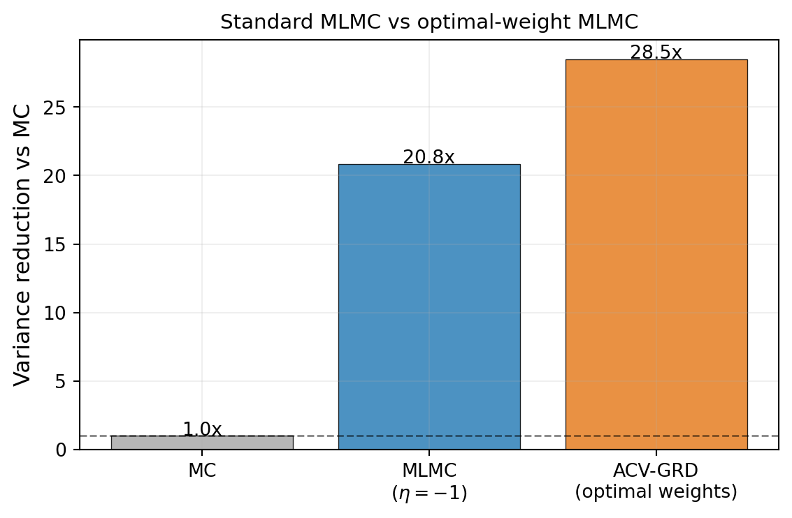
#| fig-cap: "Variance reduction relative to MC for standard MLMC ($\\eta = -1$, blue) and MLMC with optimal ACV weights (orange), at target cost $P = 500$. Optimal weights reduce variance further when the fixed-$\\eta$ structure is not optimal for this ensemble."
#| label: fig-mlmc-vs-opt
from pyapprox.statest import GRDEstimator
from pyapprox.statest.acv.allocation import ACVAllocator
from pyapprox.optimization.minimize.scipy.slsqp import (
    ScipySLSQPOptimizer,
)
from pyapprox_tutorials.figures._hierarchy import plot_mlmc_vs_opt

stat_true = MultiOutputMean(nqoi, bkd)
stat_true.set_pilot_quantities(bkd.asarray(cov_true))

P_cmp = 500.0
mlmc_est = MLMCEstimator(stat_true, bkd.asarray(costs))
mlmc_fitted_cmp = FittedACVEstimator(
    mlmc_est, default_allocator_factory(mlmc_est).allocate(P_cmp))
mlmc_var = float(mlmc_fitted_cmp.covariance()[0, 0])

acv_optimizer = ScipySLSQPOptimizer(maxiter=200)
ri_mlmc = bkd.asarray(np.arange(M), dtype=int)  # [0, 1, 2, 3]
acv_est = GRDEstimator(stat_true, bkd.asarray(costs), recursion_index=ri_mlmc)
acv_allocator = ACVAllocator(acv_est, optimizer=acv_optimizer)
acv_fitted = FittedACVEstimator(acv_est, acv_allocator.allocate(P_cmp))
acv_var = float(acv_fitted.covariance()[0, 0])

mc_stat_cmp = MultiOutputMean(nqoi, bkd)
mc_stat_cmp.set_pilot_quantities(bkd.asarray(cov_true[0:1, 0:1]))
mc_est = MCEstimator(mc_stat_cmp, bkd.asarray(costs[0:1]))
mc_fitted_cmp = MCAllocator(mc_est).allocate(P_cmp)
mc_var = float(mc_fitted_cmp.covariance()[0, 0])

labels = ["MC", "MLMC\n($\\eta=-1$)", "ACV-GRD\n(optimal weights)"]
vals   = [mc_var / mc_var, mc_var / mlmc_var, mc_var / acv_var]
colors = ["#aaaaaa", "#2C7FB8", "#E67E22"]

fig, ax = plt.subplots(figsize=(6, 4))
plot_mlmc_vs_opt(labels, vals, colors, ax)
plt.tight_layout()
plt.show()
```
::: {.callout-note}
## Pilot estimation and ACV weights
The comparison above uses the **exact** covariance from the benchmark. In practice,
the covariance is estimated from pilot samples, which introduces noise into the ACV
weight estimates. Because MLMC fixes its weights at $\eta = -1$ (no estimation needed),
it is robust to pilot noise. ACV methods that optimise weights can suffer when the
pilot is small: the estimated optimal weights may differ enough from the true optimum
that the realised variance reduction is less than predicted — or even worse than MLMC.
The advantage of optimised weights grows more reliable as the pilot size increases.
:::
## Key Takeaways
- The optimal allocation is $N_\ell^* \propto \sqrt{V_\ell / C_\ell}$, balancing high
correction variance (needs more samples) against high cost (cannot afford more samples)
- The minimum cost for target variance $\epsilon^2$ is
$C_{\text{tot}}^* = \epsilon^{-2}\bigl(\sum_\ell \sqrt{V_\ell C_\ell}\bigr)^2$
- Both MLMC and MC scale as $\epsilon^{-2}$, but the MLMC constant is much smaller when
level corrections are cheap to estimate
- MLMC fixes $\eta = -1$; optimising the weight (MLMC-OPT / ACV) can reduce variance
further when this constraint is not tight
## Exercises
1. Using the formula @eq-optimal-N, show that $N_\ell^* C_\ell \propto \sqrt{V_\ell C_\ell}$,
i.e. the fraction of total cost spent on each level is proportional to $\sqrt{V_\ell C_\ell}$.
What does this imply for the level that dominates the total cost?
2. If $V_\ell = V_0$ and $C_\ell = C_0$ for all $\ell$ (all levels identical), what does
the optimal MLMC allocation reduce to? Is it better or worse than single-level MC?
3. From @eq-min-cost, derive the condition on $\alpha$ and $\beta$ (the variance decay and
cost growth exponents) under which MLMC achieves a smaller constant than plain MC.
4. **(Challenge)** For the polynomial benchmark, compute the optimal allocation
analytically using @eq-optimal-N and compare it to the output of the allocator
from the PyApprox API. Are they consistent?
## References
- [GAN2015] M.B. Giles. *Multilevel Monte Carlo methods.* Acta Numerica, 24:259--328, 2015.
[DOI](https://doi.org/10.1017/S096249291500001X)
- [GOR2008] M.B. Giles. *Multilevel Monte Carlo path simulation.* Operations Research,
56(3):607--617, 2008. [DOI](https://doi.org/10.1287/opre.1070.0496)
- [CGSTCVS2011] K.A. Cliffe, M.B. Giles, R. Scheichl, A.L. Teckentrup. *Multilevel Monte
Carlo methods and applications to elliptic PDEs with random coefficients.* Computing and
Visualization in Science, 14:3--15, 2011.
[DOI](https://doi.org/10.1007/s00791-011-0160-x)