
From Data to Parameters: Introduction to Bayesian Inference
PyApprox Tutorial Library
Using experimental measurements to update our beliefs about uncertain model parameters.
TipDownload Notebook
Learning Objectives
After completing this tutorial, you will be able to:
- Explain why observed data motivates updating a prior distribution
- State Bayes’ theorem and identify the role of the prior, likelihood, and posterior
- Construct a likelihood function from a model and noisy observations
- Compute a posterior distribution on a grid for a one-parameter problem
- Describe how additional observations narrow the posterior
- Recognize the computational challenges that motivate MCMC and surrogate-based inference
Prerequisites
Complete Forward Uncertainty Quantification before this tutorial.
Flipping the Arrow
The forward UQ tutorial solved this problem: given a distribution over the Young’s modulus \(E\), propagate it through the beam model to get a distribution over the tip deflection \(\delta_{\text{tip}}\). The arrow pointed from parameters to predictions:
\[ \text{prior on } E \;\xrightarrow{\;f\;}\; \text{distribution on } \delta_{\text{tip}} \]
But now suppose we go to the lab and measure the tip deflection. We observe a value \(y_{\text{obs}}\). This measurement contains information about \(E\) — after all, a stiffer beam deflects less. Can we use this data to sharpen our knowledge of \(E\)?
This is the inverse problem: the arrow points backwards, from observations to parameters:
\[ \text{observation } y_{\text{obs}} \;\xrightarrow{\;?\;}\; \text{updated belief about } E \]
Bayesian inference provides the mathematical framework for flipping this arrow. Figure 1 contrasts the two directions.
Setup: The Beam Model
We use the same Euler-Bernoulli beam from the forward UQ tutorial. The tip deflection under a linearly increasing distributed load is:
\[ \delta_{\text{tip}} = f(E) = \frac{11\, q_0\, L^4}{120\, E\, I} \]
with fixed values \(q_0 = 10\), \(L = 100\), \(I = H^3/12\), \(H = 30\). The only uncertain parameter is \(E\).
from pyapprox.util.backends.numpy import NumpyBkd
from pyapprox_benchmarks.functions.algebraic.cantilever_beam import (
    HomogeneousBeam1DAnalytical,
)

bkd = NumpyBkd()

# Beam parameters (matching forward UQ tutorial)
L, H, q0 = 100.0, 30.0, 10.0

beam_model = HomogeneousBeam1DAnalytical(
    length=L, height=H, q0=q0, bkd=bkd,
)
Our prior belief about \(E\) is a Gaussian, encoding what we know from the manufacturer’s data sheet before any testing:
\[ E \sim \mathcal{N}(\mu_{\text{prior}},\, \sigma_{\text{prior}}^2) = \mathcal{N}(12{,}000,\; 2{,}000^2) \]
from pyapprox.probability.univariate.gaussian import GaussianMarginal

mu_prior = 12_000
sigma_prior = 2_000
prior = GaussianMarginal(mean=mu_prior, stdev=sigma_prior, bkd=bkd)
Generating Synthetic Data
To see Bayesian inference in action, we create a controlled experiment. We pick a “true” parameter value, run the model, and add measurement noise to produce a synthetic observation — mimicking what would happen in a real experiment.
from pyapprox.probability.likelihood import (
    DiagonalGaussianLogLikelihood,
    ModelBasedLogLikelihood,
)
from pyapprox.interface.functions.fromcallable.function import (
    FunctionFromCallable,
)

# The "true" parameter (unknown in practice)
E_true = 10_000

# True (noise-free) tip deflection
delta_true = float(beam_model(bkd.asarray([[E_true]]))[0, 0])
print(f"True E:              {E_true}")
print(f"True tip deflection: {delta_true:.6f}")

# Measurement noise: Gaussian with known standard deviation
sigma_noise = 0.4
noise_variances = bkd.asarray([sigma_noise**2])
noise_likelihood = DiagonalGaussianLogLikelihood(noise_variances, bkd)

# Wrap beam model to output only tip deflection (1 QoI out of 3)
tip_model = FunctionFromCallable(
    nqoi=1, nvars=1,
    fun=lambda E: beam_model(E)[0:1, :],
    bkd=bkd,
)

# Compose model + noise into a single parameter-to-likelihood object
model_likelihood = ModelBasedLogLikelihood(tip_model, noise_likelihood, bkd)

# Generate a synthetic observation by sampling from the likelihood
np.random.seed(42)
y_obs = float(model_likelihood.rvs(bkd.asarray([[E_true]])))
print(f"Observed deflection: {y_obs:.6f}")
print(f"Noise std dev:       {sigma_noise}")
True E: 10000
True tip deflection: 4.074074
Observed deflection: 4.272760
Noise std dev: 0.4
NoteInverse crime
We generated the data from the same model we will use for inference. In a real problem, the model is only an approximation of reality, so the “true” data-generating process differs from the model. Using the same model for both is called an inverse crime — it makes inference look easier than it really is. We use it here for pedagogical clarity.
Why Not Just Invert the Model?
With one parameter and one measurement, it is tempting to simply solve for \(E\):
\[ E = \frac{11\, q_0\, L^4}{120\, y_{\text{obs}}\, I} \]
I_rect = H**3 / 12.0
E_point_estimate = (11 * q0 * L**4) / (120 * y_obs * I_rect)
print(f"Point estimate of E: {E_point_estimate:.1f}")
print(f"True E:              {E_true}")
Point estimate of E: 9535.0
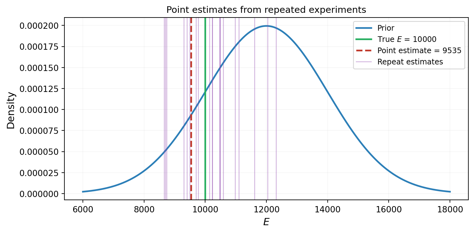
True E: 10000This gives a single number — a point estimate. But it ignores two important facts:
- The measurement is noisy: a different experiment would give a different \(y_{\text{obs}}\) and therefore a different \(E\).
- We had prior information about \(E\) before the experiment. The point estimate throws this away.
What we want is not a single number, but an updated distribution over \(E\) that combines what we knew before (the prior) with what the data tells us (the likelihood). Figure 2 illustrates why a point estimate is insufficient.
The Likelihood Function
The measurement model is:
\[ y_{\text{obs}} = f(E) + \varepsilon, \qquad \varepsilon \sim \mathcal{N}(0, \sigma_{\text{noise}}^2) \]
For a given \(E\), the probability of observing \(y_{\text{obs}}\) is:
\[ \mathcal{L}(E) = p(y_{\text{obs}} \mid E) = \frac{1}{\sqrt{2\pi}\,\sigma_{\text{noise}}} \exp\!\left(-\frac{(y_{\text{obs}} - f(E))^2}{2\,\sigma_{\text{noise}}^2}\right) \]
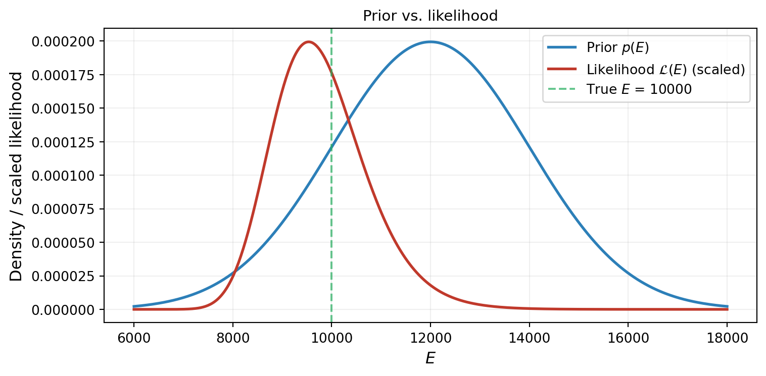
This is called the likelihood function. It is not a probability distribution over \(E\) — it is the probability of the data, evaluated as a function of \(E\). It peaks at the value of \(E\) that makes the model prediction closest to the observation.
Figure 3 shows the likelihood alongside the prior. The likelihood is concentrated near \(E \approx 10{,}000\) (where \(f(E) \approx y_{\text{obs}}\)), while the prior is centered at \(E = 12{,}000\). The data is pulling us away from our prior belief.
Bayes’ Theorem
Bayes’ theorem tells us how to combine the prior and the likelihood into an updated distribution — the posterior:
\[ \underbrace{p(E \mid y_{\text{obs}})}_{\text{posterior}} = \frac{\overbrace{\mathcal{L}(E)}^{\text{likelihood}} \;\times\; \overbrace{p(E)}^{\text{prior}}}{\underbrace{p(y_{\text{obs}})}_{\text{evidence}}} \tag{1}\]
The evidence \(p(y_{\text{obs}}) = \int \mathcal{L}(E)\, p(E)\, dE\) is a normalizing constant that ensures the posterior integrates to one. Because this integral is an expectation with respect to the prior, we can evaluate it accurately with Gauss quadrature: a small set of carefully chosen points and weights that exactly integrate polynomials of high degree.
The intuition is simple: the posterior is high where both the prior and the likelihood are high. Where the prior thinks \(E\) is plausible and the data agrees, we have high posterior probability.
from pyapprox.surrogates.quadrature import gauss_quadrature_rule

# Gauss quadrature rule for the prior: points and probability-measure weights
nquad = 50
quad_points, quad_weights = gauss_quadrature_rule(prior, nquad, bkd)
# quad_points: (1, nquad), quad_weights: (nquad, 1)

# Evaluate likelihood at quadrature points
log_lik_quad = model_likelihood.logpdf_vectorized(
    quad_points, np.array([[y_obs]]),
)  # shape (nquad, 1)
lik_quad = np.exp(log_lik_quad[:, 0])   # shape (nquad,)

# Evidence = sum of weights * likelihood (prior is absorbed in the weights)
evidence = float(lik_quad @ quad_weights[:, 0])

# Evaluate posterior on a fine grid for plotting
E_grid = np.linspace(6_000, 18_000, 500)
prior_vals = prior.pdf(E_grid[np.newaxis, :])[0, :]
log_lik_vals = model_likelihood.logpdf_vectorized(
    E_grid[np.newaxis, :], np.array([[y_obs]]),
)  # shape (ngrid, 1)
likelihood_vals = np.exp(log_lik_vals[:, 0])
posterior_vals = likelihood_vals * prior_vals / evidence

print(f"Evidence (normalizing constant): {evidence:.6e}")
Evidence (normalizing constant): 2.479322e-01Figure 4 shows the result: the posterior sits between the prior and the likelihood, shifted toward the data but tempered by the prior.

Several things to notice:
- The posterior is narrower than the prior: the data has reduced our uncertainty about \(E\).
- The posterior mean is shifted from the prior mean (\(12{,}000\)) toward the data-consistent value (\(\approx 10{,}000\)): the observation has updated our belief.
- The true value falls within the posterior’s support: the inference is working correctly.
# Posterior summary statistics via quadrature
# E[E | y] = sum_i w_i * E_i * L(E_i) / evidence
posterior_mean = float(
    (quad_points[0, :] * lik_quad) @ quad_weights[:, 0] / evidence
)
posterior_var = float(
    ((quad_points[0, :] - posterior_mean)**2 * lik_quad)
    @ quad_weights[:, 0] / evidence
)
posterior_std = np.sqrt(posterior_var)

print(f"Prior:     mean = {mu_prior},  std = {sigma_prior}")
print(f"Posterior: mean = {posterior_mean:.0f},  std = {posterior_std:.0f}")
print(f"True E:    {E_true}")
Prior: mean = 12000, std = 2000
Posterior: mean = 10206, std = 953
True E: 10000The Roles of Prior, Likelihood, and Noise
To build intuition, Figure 5 shows how the posterior changes as we vary the relative strength of the prior and the data.

This illustrates a fundamental property of Bayesian inference: the posterior is a compromise between the prior and the data, weighted by their relative precision. When the data is informative (low noise, strong likelihood), the posterior follows the data. When the prior is informative (low \(\sigma_{\text{prior}}\)), the posterior resists the data. In the limit of infinite data or zero noise, the prior becomes irrelevant and the posterior converges to the truth.
More Data, Narrower Posterior
So far we used a single observation. What happens when we collect more measurements? Each observation contributes its own likelihood. For independent observations, the joint likelihood is the product:
\[ \mathcal{L}(E \mid y_1, y_2) = p(y_1 \mid E) \cdot p(y_2 \mid E) \]
Figure 6 shows the posterior after one and two observations. The second observation further narrows the posterior and shifts it closer to the true value.

With each new observation, the posterior concentrates further around the true value. This is the Bayesian learning loop: data → update → reduced uncertainty → more data → further update.
From Posterior to Forward UQ
Once we have a posterior distribution, we can propagate it forward through the model — exactly as in the forward UQ tutorial, but now using the posterior instead of the prior. Figure 7 compares the push-forward distributions under the prior and the posterior.
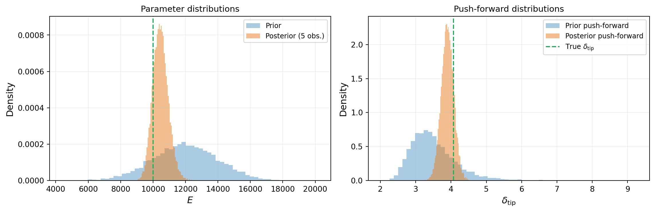
The posterior push-forward is dramatically narrower: the data has reduced our uncertainty about \(E\), which propagates to reduced uncertainty about the QoI. This is the payoff of Bayesian inference for engineering: better predictions from data-informed parameter distributions.
What We Defer
This tutorial used a 1D grid to compute the posterior exactly. This was possible because we had a single parameter. With two or more parameters, the grid approach becomes impractical: a grid with 500 points per dimension requires \(500^d\) model evaluations, which is infeasible even for \(d = 3\).
The subsequent tutorials introduce methods that scale to higher dimensions:
- Markov chain Monte Carlo (MCMC): generates samples from the posterior without evaluating it on a grid
- Surrogate-accelerated inference: replaces the expensive model \(f(E)\) with a cheap PCE approximation, making each likelihood evaluation nearly free
- Model discrepancy: accounts for the fact that the real data-generating process differs from the model
NoteThe grid approach was exact
For one parameter, grid evaluation with trapezoidal integration gives the exact posterior (up to discretization). Everything we showed in this tutorial — the prior, the likelihood, the posterior, the sequential update — is the real Bayesian posterior, not an approximation. MCMC is needed only because the grid approach does not scale, not because it is conceptually different.
Key Takeaways
- Bayesian inference updates a prior distribution using observed data to produce a posterior distribution via Bayes’ theorem: posterior \(\propto\) likelihood \(\times\) prior
- The likelihood function \(\mathcal{L}(E) = p(y_{\text{obs}} \mid E)\) measures how well each parameter value explains the data
- The posterior is a compromise between prior and data, weighted by their relative precision
- More observations narrow the posterior and push it toward the truth
- The posterior can be propagated forward through the model to produce data-informed predictions with reduced uncertainty
- Grid evaluation is exact but limited to low-dimensional problems; higher dimensions require MCMC or surrogate-based methods
Exercises
Change the true parameter to \(E_{\text{true}} = 14{,}000\) (above the prior mean instead of below). How does the posterior change? Is the posterior mean above or below the prior mean?
Increase the noise standard deviation to \(\sigma_{\text{noise}} = 4.0\) (10× larger). How does this affect the posterior after one observation? After five? How many observations are needed to recover the same posterior width as the low-noise case?
Replace the Gaussian prior with a uniform prior on \([5{,}000,\; 20{,}000]\). Compute the posterior on a grid. How does the shape differ from the Gaussian prior case? What happens in the tails?
(Challenge) With two observations \(y_1, y_2\), show that updating sequentially (prior → posterior after \(y_1\) → posterior after \(y_2\)) gives the same result as updating with both observations at once (prior → posterior after \(\{y_1, y_2\}\)). This is the sequential property of Bayesian inference.
Next Steps
Continue with:
- Markov Chain Monte Carlo — Sampling the posterior in higher dimensions