
Forward Uncertainty Quantification
PyApprox Tutorial Library
The forward UQ problem: propagating input uncertainty through a model to characterize output uncertainty.
TipDownload Notebook
Learning Objectives
After completing this tutorial, you will be able to:
- Define the forward UQ problem and its components: model, input distribution, and push-forward distribution
- Explain how input uncertainty propagates through a model to produce output uncertainty
- Recognize that different input distributions produce different output distributions, and different models do the same
- Interpret the push-forward PDF as a complete characterization of output uncertainty
- Identify common summary statistics (mean, variance, quantiles, failure probability) and explain what decisions they support
Prerequisites
Complete From Models to Decisions Under Uncertainty before this tutorial.
The Forward UQ Problem
The previous tutorial established that model inputs are uncertain and that this uncertainty propagates to the Quantity of Interest. Forward UQ is the mathematical framework for making that propagation precise.
The setup has three ingredients:
A model \(f\) that maps a parameter vector \(\params \in \Reals{\dparams}\) to a scalar QoI \(q \in \mathbb{R}\): \[ q = f(\params) \]
An input distribution \(\pdf(\params)\) — a probability density function that encodes what we know (and don’t know) about the parameters.
The push-forward distribution — the probability distribution of \(q\) induced by pushing \(\pdf(\params)\) through \(f\). This is the object we want to characterize.
Figure 1 illustrates the idea: an input distribution over \(\params\) is mapped through the model to produce an output distribution over the QoI.
NoteTerminology
The output distribution is called the push-forward because the model \(f\) “pushes” the input probability measure \(\pdf(\params)\) forward to the output space.
A Linear Model: Uncertain Loading
The simplest forward UQ problem arises when the model is a linear function of the uncertain inputs. For our cantilever beam, consider the case where the only uncertainty is in the applied load magnitude \(q_0\). The tip deflection of an Euler-Bernoulli beam under a linearly increasing distributed load is:
\[ \delta_{\text{tip}} = \underbrace{\frac{11\, L^4}{120\, EI}}_{=\, c}\; q_0 = c\, q_0 \]
This is a linear function of \(q_0\): doubling the load doubles the deflection. If \(q_0\) is drawn from a \(\normal\) distribution, the distribution of \(\delta_{\text{tip}}\) is simply a rescaled \(\normal\) — the shape is preserved and only the location and scale change. Figure 2 illustrates this.
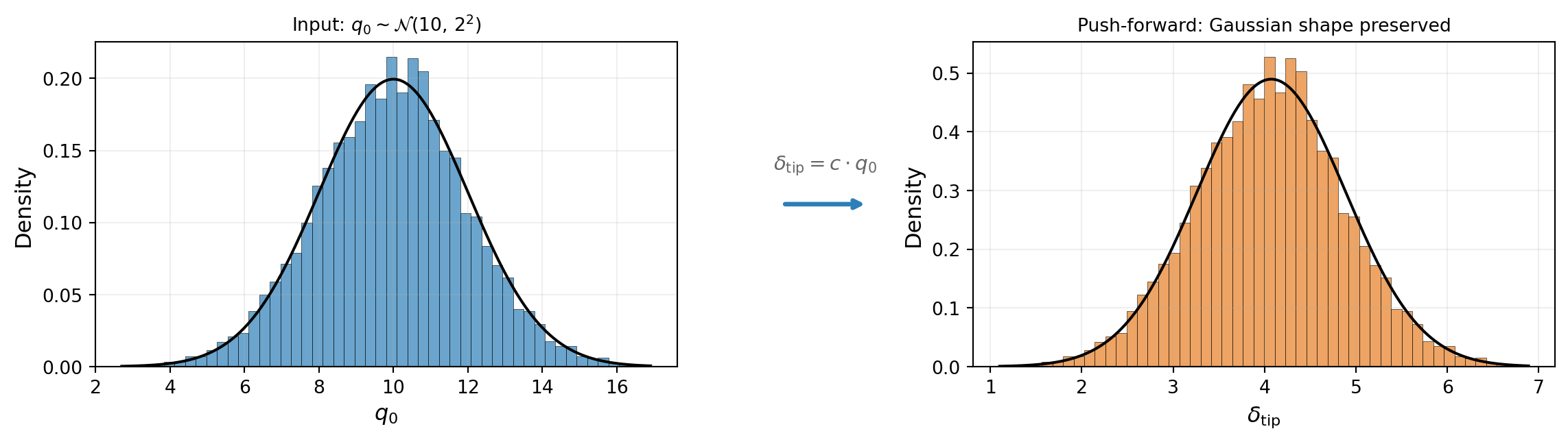
The key observation: because the model is linear, the push-forward inherits the shape of the input distribution. A \(\normal\) input produces a \(\normal\) output; a uniform input would produce a uniform output. This simple relationship breaks down for nonlinear models.
A Nonlinear Model: Uncertain Material Properties
Now consider a more realistic scenario. Fix the load at its nominal value \(q_0 = 10\) and instead treat the effective Young’s modulus \(E\) as uncertain. The tip deflection is:
\[ \delta_{\text{tip}} = \frac{11\, q_0\, L^4}{120\, E I} \propto \frac{1}{E} \]
This is a nonlinear function of \(E\): the relationship \(\delta_{\text{tip}} \propto 1/E\) means that a symmetric distribution on \(E\) produces an asymmetric distribution on \(\delta_{\text{tip}}\). Small values of \(E\) cause disproportionately large deflections.
Figure 3 illustrates this. Even though the input distribution on \(E\) is symmetric (\(\normal\)), the output distribution is right-skewed. The nonlinearity of the model has distorted the shape.
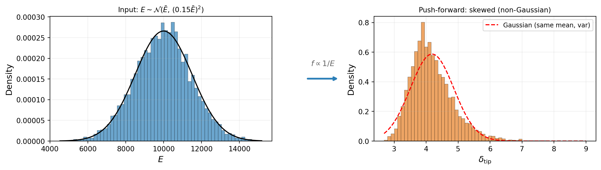
This is the generic situation in UQ: most models of interest are nonlinear, so the push-forward distribution has a different shape than the input, and its properties cannot be deduced from the input distribution alone — they must be computed.
Different Inputs and Models Produce Different Push-Forwards
Two factors determine the push-forward distribution: the input distribution and the model. Changing either one changes the output.
Figure 4 shows the same beam model evaluated with two different input distributions on \(E\): a narrow one (low uncertainty) and a wide one (high uncertainty). The push-forward distributions differ in both spread and shape — the wider input produces a heavier right tail because the \(1/E\) nonlinearity amplifies low-stiffness samples.
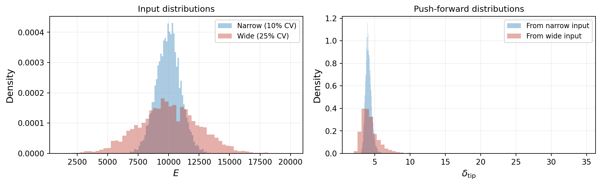
Figure 5 shows the complementary effect: the same input distribution evaluated with two different models. Both use the Euler-Bernoulli formula but with different beam lengths:
\[ f_1(E) = \frac{11\, q_0\, L_1^4}{120\, E\, I}, \qquad f_2(E) = \frac{11\, q_0\, L_2^4}{120\, E\, I} \]
Because deflection scales as \(L^4\), even a modest change in length significantly shifts the push-forward distribution. Both models receive identical random samples of \(E\), but produce different outputs.
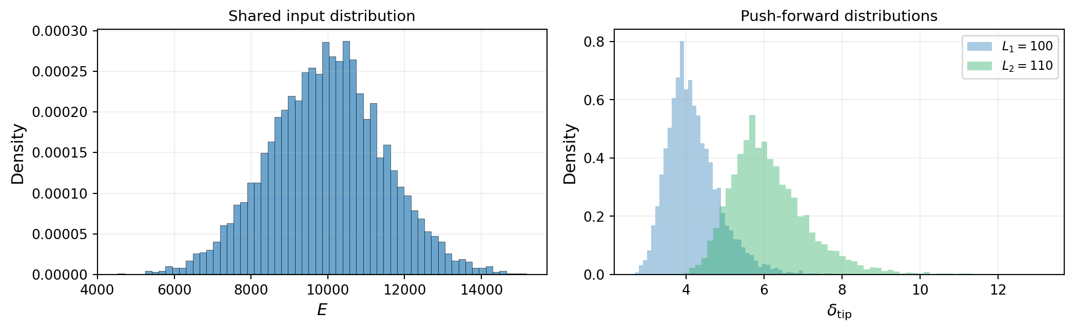
These two figures illustrate a fundamental point: the push-forward distribution depends on both the input distribution and the model. Getting either one wrong changes the conclusions. This is why UQ must address parameter uncertainty and model-form uncertainty as complementary concerns.
The Push-Forward PDF and Summary Statistics
The push-forward distribution \(\pdf_q(q)\) is the complete answer to the forward UQ problem — it tells us the probability of every possible value of the QoI. In principle, if we know this density, we know everything.
In practice, however, decision makers rarely need the full PDF. They need specific numbers that answer specific questions. Figure 6 illustrates the most common summary statistics extracted from a push-forward distribution:

Each statistic answers a different question:
- Mean \(\E_{\params}[q]\): What is the average prediction? Useful for design targets and expected performance.
- Variance \(\Var_{\params}[q]\) (or standard deviation \(\sigma\)): How spread out are the predictions? Quantifies overall uncertainty.
- Quantile interval (e.g., 5th to 95th percentile): What range contains 90% of plausible outcomes? Useful for confidence bounds and safety margins.
- Failure probability \(P(q > q_{\text{crit}})\): How likely is it that the QoI exceeds a critical threshold? Directly relevant to certification and risk assessment.
ImportantPDF vs. summary statistics
The push-forward PDF contains all the information — every summary statistic can be derived from it. But the PDF itself is expensive to estimate accurately (it requires many model evaluations). In practice, UQ methods often target specific statistics directly, which can be far cheaper than reconstructing the full distribution.
Key Takeaways
- Forward UQ propagates a known input distribution \(\pdf(\params)\) through a model \(f\) to produce a push-forward distribution over the QoI
- A linear model preserves the shape of the input distribution; a nonlinear model distorts it, so the output distribution must be computed rather than assumed
- The push-forward depends on both the input distribution and the model — changing either one changes the conclusions
- The push-forward PDF \(\pdf_q(q)\) is the complete characterization of output uncertainty, but decision makers typically extract summary statistics: \(\E_{\params}[q]\), \(\Var_{\params}[q]\), quantile intervals, and failure probabilities
- Computing these statistics for expensive models is the central computational challenge of UQ — the subsequent tutorials introduce methods for doing so efficiently
Notation Summary
| Symbol | Meaning |
|---|---|
| \(\params\) | Parameter vector \((\theta_1, \ldots, \theta_{\dparams})\) |
| \(\dparams\) | Number of uncertain parameters |
| \(f(\params)\) | Forward model (maps parameters to QoI) |
| \(q = f(\params)\) | Quantity of Interest (scalar output) |
| \(\pdf(\params)\) | Input probability density function |
| \(\pdf_q(q)\) | Push-forward (output) density |
| \(\E_{\params}[\cdot]\) | Expected value with respect to \(\params\) |
| \(\Var_{\params}[\cdot]\) | Variance with respect to \(\params\) |
| \(\normal(\mu, \sigma^2)\) | Gaussian distribution |
| \(P(q > q_{\text{crit}})\) | Failure probability |
Next Steps
Continue with:
- Random Variables & Distributions — Specifying input distributions mathematically
- Monte Carlo Sampling — The simplest method for estimating push-forward statistics
- Sensitivity Analysis — Identifying which inputs dominate the output uncertainty