---
title: "The Surrogate Modeling Workflow"
subtitle: "PyApprox Tutorial Library"
description: "Build your first surrogate model and learn the four-step workflow that every surrogate method follows."
tutorial_type: conceptual
topic: surrogate_modeling
difficulty: beginner
estimated_time: 10
prerequisites:
- setup_environment
tags:
- surrogate
- workflow
- polynomial
- least-squares
format:
html:
code-fold: false
code-tools: true
toc: true
execute:
echo: true
warning: false
jupyter: python3
---
::: {.callout-tip collapse="true"}
## Download Notebook
[Download as Jupyter Notebook](notebooks/surrogate_workflow.ipynb)
:::
## Learning Objectives
After completing this tutorial, you will be able to:
- Explain why surrogate models are needed for expensive simulators
- Describe the four-step surrogate workflow: ansatz, data, fitting, assessment
- Distinguish continuous $L_2$ minimisation from its discrete approximation
- Fit a polynomial surrogate to sampled data using least squares
- Assess surrogate accuracy on an independent test set
- Interpret a convergence plot to judge whether the surrogate has converged
## The Cost Problem
Computational models in engineering and science can take minutes, hours, or days per
evaluation. When we want to understand how uncertain inputs affect the model outputs ---
computing means, variances, failure probabilities --- we need hundreds to thousands of
evaluations. A Monte Carlo estimate of the mean converges only as $1/\sqrt{N}$;
estimating variances or tail probabilities requires even more samples.
The idea behind a **surrogate model** is simple: replace the expensive simulator
$f(\mathbf{x})$ with a cheap approximation $\hat{f}(\mathbf{x})$ that can be evaluated
millions of times at negligible cost. We invest a modest number of expensive model
evaluations to *train* the surrogate, then use it as a stand-in for all subsequent
analysis.
Every surrogate method --- polynomial expansions, Gaussian processes, function trains,
neural networks --- follows the same four-step workflow:
1. **Choose an ansatz** --- the functional form $\hat{f}$ will take
2. **Collect training data** --- evaluate the expensive model at selected input points
3. **Fit the surrogate** --- find the parameters of $\hat{f}$ that best match the data
4. **Assess and use** --- verify accuracy, then deploy for downstream analysis
This tutorial walks through each step on a concrete 1D example. The concepts and figures
here apply to every surrogate type you will encounter later.
## The True Function
We need a function that is cheap enough to evaluate densely (so we can see the ground
truth) but rich enough to require a nontrivial surrogate. We use
$$
f(x) = \sin(1.5\pi x)\,e^{-x^2}
$$
on $x \in [-1, 1]$. It is smooth, oscillatory, and has an amplitude envelope that varies
across the domain --- a polynomial will need several terms to capture it.
```{python}
#| fig-cap: "The function we want to approximate. In a real application this curve would be unknown --- we could only see it at the handful of points where we can afford to run the expensive model."
#| label: fig-true-function
import numpy as np
import matplotlib.pyplot as plt
from pyapprox.util.backends.numpy import NumpyBkd
from pyapprox.interface.functions.fromcallable.function import FunctionFromCallable

bkd = NumpyBkd()

def _f_true(samples):
    x = samples[0:1, :]
    return bkd.sin(1.5 * np.pi * x) * bkd.exp(-x**2)

model = FunctionFromCallable(nqoi=1, nvars=1, fun=_f_true, bkd=bkd)

x_dense = np.linspace(-1, 1, 500)
x_dense_2d = bkd.asarray(x_dense.reshape(1, -1))
f_dense = bkd.to_numpy(model(x_dense_2d)).ravel()

fig, ax = plt.subplots(figsize=(7, 3.5))
ax.plot(x_dense, f_dense, "k-", lw=2, label=r"$f(x)$")
ax.set_xlabel(r"$x$")
ax.set_ylabel(r"$f(x)$")
ax.legend()
ax.set_title("True function")
plt.tight_layout()
plt.show()
```
In a real application we would *not* have this dense curve. We would only be able to see
$f$ at a handful of points where we can afford to run the expensive model. The surrogate's
job is to fill in everything in between.
## Step 1: Choose an Ansatz
The **ansatz** is the functional form we assume for the surrogate. Here we choose a
polynomial:
$$
\hat{f}(x) = \sum_{j=0}^{p} c_j\, \phi_j(x)
$$
where $\phi_j$ are polynomial basis functions and $c_j$ are coefficients we will
determine from data. The **degree** $p$ controls how flexible the surrogate can be.
A polynomial is a natural first choice: it is simple, well understood, and for smooth
functions converges rapidly as $p$ increases. But the ansatz imposes a hard constraint ---
$\hat{f}$ *cannot* represent anything outside the span of $\{\phi_0, \ldots, \phi_p\}$.
If the true function has features that polynomials struggle with (discontinuities,
sharp kinks), no amount of data or clever fitting will fix the problem. Choosing an
appropriate ansatz is the most consequential decision in the entire workflow;
[What Makes a Good Surrogate?](surrogate_design.qmd) explores this in detail.
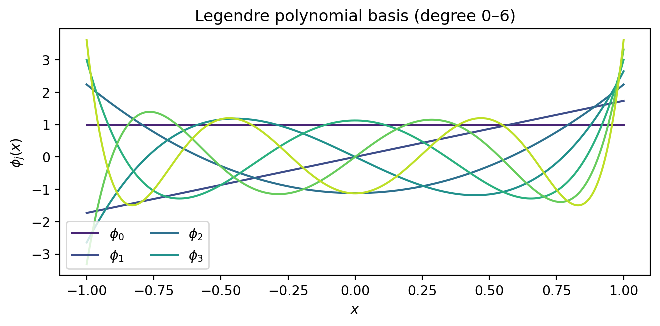
Let us visualise what basis functions are available at degree $p = 6$:
```{python}
#| fig-cap: "Legendre polynomial basis functions up to degree 6. Any degree-6 polynomial surrogate is a weighted combination of these seven functions. The surrogate can only represent shapes that lie in the span of this basis."
#| label: fig-basis-functions
from pyapprox.probability import UniformMarginal
from pyapprox.surrogates.affine.expansions import create_pce_from_marginals

marginals = [UniformMarginal(-1.0, 1.0, bkd)]

pce_basis = create_pce_from_marginals(marginals, max_level=6, bkd=bkd, nqoi=1)
Phi_dense = bkd.to_numpy(pce_basis.basis_matrix(x_dense_2d))   # (500, 7)

fig, ax = plt.subplots(figsize=(7, 3.5))
colors = plt.cm.viridis(np.linspace(0.1, 0.9, 7))
for j in range(7):
    ax.plot(x_dense, Phi_dense[:, j], color=colors[j], lw=1.5,
            label=rf"$\phi_{j}$" if j < 4 else None)
ax.set_xlabel(r"$x$")
ax.set_ylabel(r"$\phi_j(x)$")
ax.legend(loc="lower left", ncol=2)
ax.set_title(f"Legendre polynomial basis (degree 0–6)")
plt.tight_layout()
plt.show()
```
## Step 2: Collect Training Data
To fit the surrogate we need **training data**: pairs
$\{(x^{(i)},\, f(x^{(i)}))\}_{i=1}^{N}$ obtained by evaluating the expensive model.
The simplest strategy is to draw $N$ points at random from the input domain.
```{python}
#| fig-cap: "Twenty random training points sampled from the true function. In a real problem each dot represents one expensive model evaluation."
#| label: fig-training-data
np.random.seed(42)
N_train = 20
samples_tr = bkd.asarray(np.random.uniform(-1, 1, (1, N_train)))
values_tr = model(samples_tr)                       # (1, N_train)

x_train = bkd.to_numpy(samples_tr).ravel()
f_train = bkd.to_numpy(values_tr).ravel()

fig, ax = plt.subplots(figsize=(7, 3.5))
ax.plot(x_dense, f_dense, "k-", lw=1.5, alpha=0.4, label=r"$f(x)$ (unknown)")
ax.plot(x_train, f_train, "ko", ms=6, zorder=5, label="Training data")
ax.set_xlabel(r"$x$")
ax.set_ylabel(r"$f(x)$")
ax.legend()
ax.set_title(f"$N = {N_train}$ training evaluations")
plt.tight_layout()
plt.show()
```
::: {.callout-note}
## Where you sample matters
Random sampling is simple but not optimal. Some sample designs --- such as quasi-Monte
Carlo sequences or induced sampling --- give better coverage of the input space and can
dramatically improve surrogate accuracy for the same $N$.
[What Makes a Good Surrogate?](surrogate_design.qmd) discusses this in detail.
:::
## Step 3: Fit the Surrogate
### What We Want vs. What We Can Compute
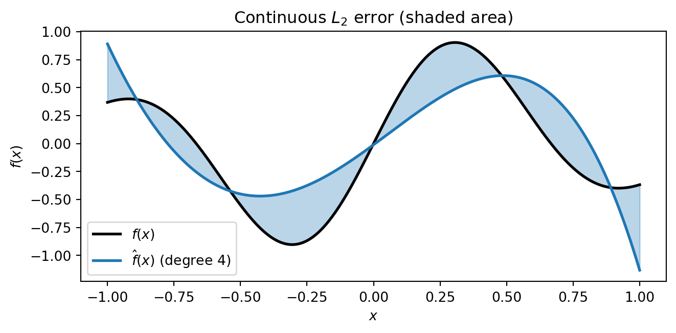
Ideally we would find coefficients $\mathbf{c}$ that minimise the **continuous $L_2$
error** --- the integrated squared difference between the surrogate and the true function
over the entire domain:
$$
\|\hat{f} - f\|_{L_2}^2 = \int_{-1}^{1} \bigl[\hat{f}(x) - f(x)\bigr]^2 \, dx
$$
```{python}
#| echo: false
#| fig-cap: "What we want to minimise: the continuous L₂ error. The shaded area between the surrogate and the true function represents the integrated squared difference over the whole domain. Computing this requires knowing f(x) everywhere — which is exactly what we do not have."
#| label: fig-continuous-l2
from pyapprox.surrogates.affine.expansions.fitters import LeastSquaresFitter
# Rough surrogate for illustration (deliberately mediocre fit)
degree_demo = 4
pce_demo = create_pce_from_marginals(marginals, max_level=degree_demo, bkd=bkd, nqoi=1)
samples_tr = bkd.asarray(x_train.reshape(1, -1))
values_tr = bkd.asarray(f_train.reshape(1, -1))
ls_fitter = LeastSquaresFitter(bkd)
result_demo = ls_fitter.fit(pce_demo, samples_tr, values_tr)
pce_demo = result_demo.surrogate()
fhat_dense = bkd.to_numpy(pce_demo(x_dense_2d)).ravel()
fig, ax = plt.subplots(figsize=(7, 3.5))
ax.plot(x_dense, f_dense, "k-", lw=2, label=r"$f(x)$")
ax.plot(x_dense, fhat_dense, "C0-", lw=2, label=rf"$\hat{{f}}(x)$ (degree {degree_demo})")
ax.fill_between(x_dense, f_dense, fhat_dense, alpha=0.3, color="C0")
ax.set_xlabel(r"$x$")
ax.set_ylabel(r"$f(x)$")
ax.legend()
ax.set_title(r"Continuous $L_2$ error (shaded area)")
plt.tight_layout()
plt.show()
```
But computing this integral requires evaluating $f(x)$ everywhere --- which is exactly
what we cannot afford. Instead, we minimise the **discrete $L_2$ error** at the $N$
training points:
$$
\hat{\mathbf{c}} = \arg\min_{\mathbf{c}} \sum_{i=1}^{N}
\Bigl[ f(x^{(i)}) - \sum_{j=0}^{p} c_j\, \phi_j(x^{(i)}) \Bigr]^2
$$
```{python}
#| echo: false
#| fig-cap: "What we actually minimise: the discrete L₂ error. Each vertical bar shows the residual |f(xⁱ) − f̂(xⁱ)| at a training point. We minimise the sum of squared bar lengths — a standard least-squares problem."
#| label: fig-discrete-l2
fig, ax = plt.subplots(figsize=(7, 3.5))
ax.plot(x_dense, f_dense, "k-", lw=1.5, alpha=0.4, label=r"$f(x)$")
ax.plot(x_dense, fhat_dense, "C0-", lw=2, label=rf"$\hat{{f}}(x)$")
fhat_train = bkd.to_numpy(pce_demo(samples_tr)).ravel()
for i in range(N_train):
ax.plot([x_train[i], x_train[i]], [f_train[i], fhat_train[i]],
"C3-", lw=2, alpha=0.7)
ax.plot(x_train, f_train, "ko", ms=6, zorder=5)
ax.set_xlabel(r"$x$")
ax.set_ylabel(r"$f(x)$")
ax.legend()
ax.set_title(r"Discrete $L_2$ error (residuals at training points)")
plt.tight_layout()
plt.show()
```
The hope is that if the discrete error is small at enough well-placed training points,
the continuous error will be small too. This is exactly why the number and placement of
training points matters.
### Solving the Least-Squares Problem
In matrix form, we assemble the **basis matrix** (or Vandermonde matrix)
$\Phi_{ij} = \phi_j(x^{(i)})$ and solve:
$$
\hat{\mathbf{c}} = (\boldsymbol{\Phi}^\top \boldsymbol{\Phi})^{-1}
\boldsymbol{\Phi}^\top \mathbf{f}
$$
```{python}
degree = 6

pce = create_pce_from_marginals(marginals, max_level=degree, bkd=bkd, nqoi=1)

# Build basis matrix
Phi = pce.basis_matrix(samples_tr)     # (N_train, nterms)

# Fit via least squares
result = LeastSquaresFitter(bkd).fit(pce, samples_tr, values_tr)
pce = result.surrogate()
```
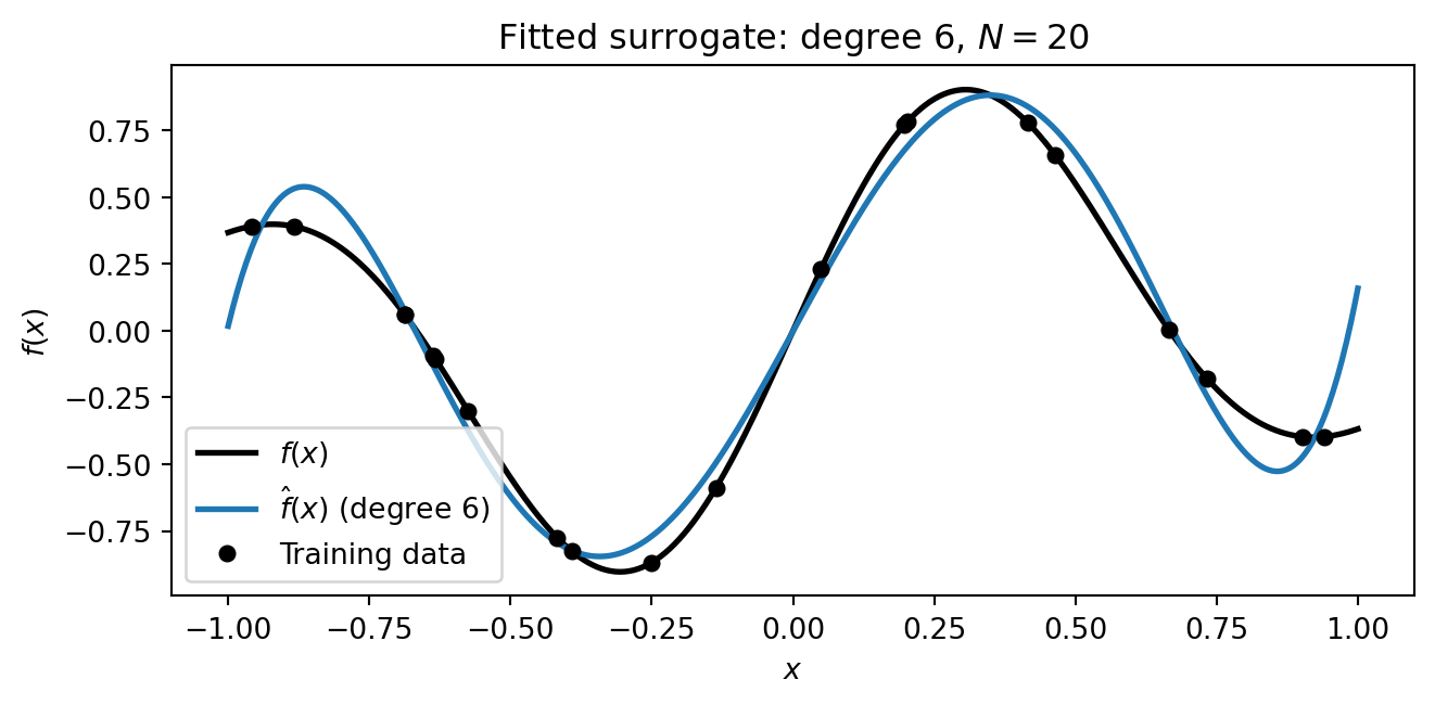
```{python}
#| fig-cap: "The fitted degree-6 polynomial surrogate (blue) overlaid on the true function (black). The surrogate captures the overall shape using only the 20 training points."
#| label: fig-fitted-surrogate
fig, ax = plt.subplots(figsize=(7, 3.5))
ax.plot(x_dense, f_dense, "k-", lw=2, label=r"$f(x)$")
pce_dense = bkd.to_numpy(pce(x_dense_2d)).ravel()
ax.plot(x_dense, pce_dense, "C0-", lw=2, label=rf"$\hat{{f}}(x)$ (degree {degree})")
ax.plot(x_train, f_train, "ko", ms=5, zorder=5, label="Training data")
ax.set_xlabel(r"$x$")
ax.set_ylabel(r"$f(x)$")
ax.legend()
ax.set_title(f"Fitted surrogate: degree {degree}, $N = {N_train}$")
plt.tight_layout()
plt.show()
```
## Step 4: Assess the Surrogate
A surrogate that fits its training data well may still be inaccurate elsewhere. We
always evaluate accuracy on an **independent test set** that was not used during fitting.
### Relative $L_2$ Error
The standard accuracy metric is the **relative $L_2$ error**:
$$
\epsilon = \frac{\| f(\mathbf{X}_{\mathrm{test}}) - \hat{f}(\mathbf{X}_{\mathrm{test}}) \|_2}
{\| f(\mathbf{X}_{\mathrm{test}}) \|_2}
$$
This normalises the error by the magnitude of the function, so $\epsilon = 10^{-3}$
means the surrogate reproduces the function to roughly 0.1% accuracy.
```{python}
np.random.seed(123)
N_test = 500
samples_test = bkd.asarray(np.random.uniform(-1, 1, (1, N_test)))
values_test = model(samples_test)

f_test = bkd.to_numpy(values_test).ravel()
fhat_test = bkd.to_numpy(pce(samples_test)).ravel()

l2_err = np.linalg.norm(f_test - fhat_test) / np.linalg.norm(f_test)
print(f"Relative L2 error: {l2_err:.4e}")
```
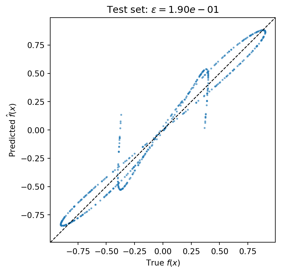
```{python}
#| echo: false
#| fig-cap: "Predicted vs. true values on the 500-point test set. Points near the diagonal indicate accurate predictions. Scatter away from the diagonal reveals where the surrogate struggles."
#| label: fig-predicted-vs-true
fig, ax = plt.subplots(figsize=(5, 5))
ax.plot(f_test, fhat_test, "C0.", ms=3, alpha=0.5)
lims = [min(f_test.min(), fhat_test.min()), max(f_test.max(), fhat_test.max())]
margin = 0.05 * (lims[1] - lims[0])
lims = [lims[0] - margin, lims[1] + margin]
ax.plot(lims, lims, "k--", lw=1)
ax.set_xlim(lims)
ax.set_ylim(lims)
ax.set_xlabel(r"True $f(x)$")
ax.set_ylabel(r"Predicted $\hat{f}(x)$")
ax.set_title(rf"Test set: $\epsilon = {l2_err:.2e}$")
ax.set_aspect("equal")
plt.tight_layout()
plt.show()
```
### Convergence: Is the Surrogate Good Enough?
A single error number does not tell us whether the surrogate has converged. The key
diagnostic is a **convergence plot**: how does the error decrease as we invest more
computational effort?
For a polynomial surrogate, two things control accuracy: the polynomial **degree** $p$
(which determines the richness of the ansatz) and the number of **training points** $N$
(which determines how well we can estimate the coefficients). We must increase both
together. Increasing $N$ at fixed $p$ will plateau at the truncation error --- the best
the degree-$p$ polynomial can achieve regardless of data. Increasing $p$ at fixed $N$
will eventually overfit.
The following convergence study increases $p$ and scales $N$ proportionally, using an
oversampling ratio of $N = 5(p+1)$:
```{python}
#| fig-cap: "Convergence of the polynomial surrogate as degree p and training set size N increase together. Each point uses N = 5(p+1) training samples. The error decreases steadily until the surrogate captures essentially all the function's structure."
#| label: fig-convergence
np.random.seed(0)

degrees = list(range(1, 16))
oversample = 5
errors = []

for p in degrees:
    N = oversample * (p + 1)
    s_tr = bkd.asarray(np.random.uniform(-1, 1, (1, N)))
    v_tr = model(s_tr)
    pce_p = create_pce_from_marginals(marginals, max_level=p, bkd=bkd, nqoi=1)
    res_p = LeastSquaresFitter(bkd).fit(pce_p, s_tr, v_tr)
    pce_p = res_p.surrogate()
    fhat_conv = bkd.to_numpy(pce_p(samples_test)).ravel()
    err = np.linalg.norm(f_test - fhat_conv) / np.linalg.norm(f_test)
    errors.append(err)

fig, ax = plt.subplots(figsize=(7, 4))
ax.semilogy(degrees, errors, "C0o-", lw=2, ms=6)
ax.set_xlabel("Polynomial degree $p$")
ax.set_ylabel(r"Relative $L_2$ error")
ax.set_title(r"Convergence: degree $p$ with $N = 5(p+1)$ training points")
ax.grid(True, alpha=0.3)

# Add secondary x-axis for N
ax2 = ax.twiny()
ax2.set_xlim(ax.get_xlim())
tick_degrees = [1, 4, 7, 10, 13]
ax2.set_xticks(tick_degrees)
ax2.set_xticklabels([f"{oversample*(p+1)}" for p in tick_degrees])
ax2.set_xlabel("Training points $N$")

plt.tight_layout()
plt.show()
```
The steady downward trend confirms that both the ansatz and the data are adequate. If
the curve **levels off** at a high error, the ansatz may be too restrictive (the
polynomial cannot represent the function well). If it **turns upward**, the surrogate is
overfitting --- see
[Overfitting and Cross-Validation](practical_pce_fitting.qmd) for how to detect and
prevent this.
### What Can We Do with the Surrogate?
Once validated, the surrogate can be evaluated millions of times at negligible cost.
This enables analyses that would be infeasible with the expensive model:
```{python}
#| fig-cap: "With the surrogate we can instantly generate dense evaluations (left) and estimate output statistics via Monte Carlo on the cheap surrogate (right) — all impossible if each evaluation took hours."
#| label: fig-postprocessing
fig, axes = plt.subplots(1, 2, figsize=(10, 3.5))

# Panel 1: Dense evaluation
ax = axes[0]
ax.plot(x_dense, f_dense, "k-", lw=1.5, alpha=0.4, label=r"$f$")
ax.plot(x_dense, pce_dense, "C0-", lw=2, label=r"$\hat{f}$")
ax.plot(x_train, f_train, "ko", ms=4, zorder=5)
ax.set_title("Dense surrogate evaluation")
ax.set_xlabel(r"$x$")
ax.legend(fontsize=9)

# Panel 2: Cheap Monte Carlo on surrogate
ax = axes[1]
N_mc = 100_000
samples_mc = bkd.asarray(np.random.uniform(-1, 1, (1, N_mc)))
fhat_mc = bkd.to_numpy(pce(samples_mc)).ravel()
ax.hist(fhat_mc, bins=60, density=True, color="C0", alpha=0.7, edgecolor="white",
        lw=0.3)
mean_est = np.mean(fhat_mc)
ax.axvline(mean_est, color="k", lw=2, ls="--", label=rf"$\mu \approx {mean_est:.3f}$")
ax.set_title("Output distribution ($10^5$ MC samples)")
ax.set_xlabel(r"$\hat{f}(x)$")
ax.legend(fontsize=9)

plt.tight_layout()
plt.show()
```
## Key Takeaways
- **Surrogate models** replace expensive simulators with cheap approximations, enabling
analyses that would otherwise be computationally infeasible.
- Every surrogate method follows the same **four-step workflow**: choose an ansatz,
collect training data, fit the surrogate, then assess accuracy.
- The **ansatz** constrains what the surrogate can represent. A polynomial works well for
smooth functions; other function structures call for other surrogate types.
- We want to minimise the **continuous $L_2$ error** but can only compute the
**discrete** version at training points. The gap between these motivates careful
sample design.
- Always assess accuracy on an **independent test set**, not the training data.
- A **convergence plot** — error vs. increasing degree and training set size — is the
essential diagnostic. Increase both together to avoid plateauing at the truncation
error.
## Next Steps
- [What Makes a Good Surrogate?](surrogate_design.qmd) --- How the choice of ansatz,
sample design, and fitting strategy affect surrogate quality, and how different
surrogates exploit different kinds of function structure
- [Building a Polynomial Chaos Surrogate](polynomial_chaos_surrogates.qmd) --- Apply the
workflow to a real engineering model using orthogonal polynomials matched to the input
distribution
- [Building a Gaussian Process Surrogate](gp_surrogate.qmd) --- A probabilistic
surrogate that provides built-in uncertainty quantification
- [An Introduction to Function Trains](function_train_surrogates.qmd) --- Exploit
low-rank structure for high-dimensional problems