import numpy as np
import matplotlib.pyplot as plt

from pyapprox.util.backends.numpy import NumpyBkd
from pyapprox.surrogates.sparsegrids import (
    SingleFidelityAdaptiveSparseGridFitter,
    TensorProductSubspaceFactory,
)
from pyapprox.surrogates.sparsegrids.basis_factory import (
    ClenshawCurtisLagrangeFactory,
    PiecewiseFactory,
)
from pyapprox.surrogates.sparsegrids.basis.hierarchical_basis_1d import (
    HierarchicalBasis1D,
)
from pyapprox.surrogates.sparsegrids.hierarchical.hierarchical_fitter import (
    SingleFidelityHierarchicalFitter,
)
from pyapprox.surrogates.affine.indices import (
    ClenshawCurtisGrowthRule,
    MaxLevelCriteria,
)
from pyapprox.probability.univariate.uniform import UniformMarginal
from pyapprox.interface.functions.fromcallable.function import (
    FunctionFromCallable,
)

bkd = NumpyBkd()
np.random.seed(0)

marginal = UniformMarginal(0.0, 1.0, bkd)
max_pts = 1000

rng = np.random.default_rng(0)
test_samples = bkd.asarray(rng.uniform(0, 1, (2, 4000)))Local Adaptivity vs Combination Technique
PyApprox Tutorial Library
Side-by-side benchmark: locally adaptive hierarchical sparse grids beat the dimension-adaptive combination technique on a non-smooth 2D target.
TipDownload Notebook
Learning Objectives
After completing this tutorial, you will be able to:
- Construct a locally adaptive sparse grid with
boundary_mode="include"andMaxLevelCriteria - Run the same convergence experiment with the dimension-adaptive combination technique using piecewise bases
- Compare the two methods on a non-smooth target with a localised feature
- Explain why local adaptivity outperforms dimension adaptivity on localised features
Prerequisites
Local Basis Sparse Grids and Locally Adaptive Sparse Grids. This tutorial uses the hierarchical fitter API from the second.
Setup
Target Function
The benchmark has a sharp, localized feature that both dimensions contribute to:
\[ f(\xi) = \frac{1}{|0.3 - \xi_1^2 - \xi_2^2| + 0.1}, \qquad \xi \in [0,1]^2. \]
The near-singularity along the curve \(\xi_1^2 + \xi_2^2 = 0.3\) creates a ridge that is not axis-aligned. Both dimensions matter, but the feature is spatially localized — exactly the setting where local adaptivity should outperform dimension adaptivity.
def _target_callable(samples):
    z1, z2 = samples[0], samples[1]
    return bkd.reshape(1.0 / (bkd.abs(0.3 - z1**2 - z2**2) + 0.1), (1, -1))

target_fn = FunctionFromCallable(1, 2, _target_callable, bkd)
exact_vals = bkd.to_numpy(target_fn(test_samples))[0]
Combination Technique (Dimension-Adaptive)
The combination technique builds the surrogate from a sum of tensor- product subspaces selected by a dimension-level error indicator. When it identifies a dimension as important it refines the entire axis to the next level — adding nodes uniformly even in regions where the function is smooth.
def make_piecewise_factories(poly_type):
    return [PiecewiseFactory(marginal, bkd, poly_type=poly_type)
            for _ in range(2)]

def make_lagrange_factories():
    return [ClenshawCurtisLagrangeFactory(marginal, bkd)
            for _ in range(2)]

def run_combination(factories, max_level=15, tol=1e-10):
    """Dimension-adaptive combination technique."""
    growth = ClenshawCurtisGrowthRule()
    tp = TensorProductSubspaceFactory(bkd, factories, growth)
    admis = MaxLevelCriteria(max_level=max_level, pnorm=1.0, bkd=bkd)
    fitter = SingleFidelityAdaptiveSparseGridFitter(bkd, tp, admis)

    ns_hist, err_hist = [], []
    while True:
        new_samples = fitter.step_samples()
        if new_samples is None:
            break
        fitter.step_values(target_fn(new_samples))
        result = fitter.result()
        if result.nsamples > 1:
            approx = bkd.to_numpy(result.surrogate(test_samples))[0]
            rmse = float(np.sqrt(np.mean((exact_vals - approx) ** 2)))
            ns_hist.append(result.nsamples)
            err_hist.append(rmse)
        if fitter.current_error() < tol or fitter.cumulative_cost() >= max_pts:
            break
    return ns_hist, err_hist
Locally Adaptive (Downward-Closed, Boundaries Included)
The locally adaptive fitter tracks per-point surpluses and refines the single point with the largest surplus next. Near the ridge those surpluses stay large while surpluses in the smooth regions decay quickly, so refinement concentrates on the ridge.
def run_local(p_max, max_level=15):
    """Locally adaptive hierarchical fitter with boundaries."""
    bases_1d = [
        HierarchicalBasis1D(bkd, bounds=(0.0, 1.0), p_max=p_max,
                            boundary_mode="include"),
        HierarchicalBasis1D(bkd, bounds=(0.0, 1.0), p_max=p_max,
                            boundary_mode="include"),
    ]
    admis = MaxLevelCriteria(max_level=max_level, pnorm=1.0, bkd=bkd)
    fitter = SingleFidelityHierarchicalFitter(
        bkd, bases_1d, admis, batch_size=1,
    )

    ns_hist, err_hist = [], []
    total = 0
    while total < max_pts:
        new_samples = fitter.step_samples()
        if new_samples is None:
            break
        fitter.step_values(target_fn(new_samples))
        total += int(new_samples.shape[1])
        result = fitter.result()
        if result.nsamples > 1:
            approx = bkd.to_numpy(result.surrogate(test_samples))[0]
            rmse = float(np.sqrt(np.mean((exact_vals - approx) ** 2)))
            ns_hist.append(result.nsamples)
            err_hist.append(rmse)
    return ns_hist, err_hist, fitter
Run the Experiments
ns_comb_lag, err_comb_lag = run_combination(make_lagrange_factories())
ns_comb_lin, err_comb_lin = run_combination(make_piecewise_factories("linear"))
ns_comb_quad, err_comb_quad = run_combination(make_piecewise_factories("quadratic"))
ns_loc_lin, err_loc_lin, fitter_loc_lin = run_local(p_max=1)
ns_loc_quad, err_loc_quad, fitter_loc_quad = run_local(p_max=2)
Convergence Comparison
fig, ax = plt.subplots(figsize=(7, 4.5))
ax.loglog(ns_comb_lag,  err_comb_lag,  "v--", color="#9467BD", lw=2,
          label="Combination, Lagrange")
ax.loglog(ns_comb_lin,  err_comb_lin,  "^--", color="#7F7F7F", lw=2,
          label="Combination, piecewise linear")
ax.loglog(ns_comb_quad, err_comb_quad, "s--", color="#E6550D", lw=2,
          label="Combination, piecewise quadratic")
ax.loglog(ns_loc_lin,   err_loc_lin,   "o-",  color="#1F77B4", lw=2,
          label="Local adaptive, $p_{\\max}=1$")
ax.loglog(ns_loc_quad,  err_loc_quad,  "D-",  color="#2CA02C", lw=2,
          label="Local adaptive, $p_{\\max}=2$")
ax.set_xlabel("Number of function evaluations")
ax.set_ylabel("RMSE on test set")
ax.set_title("$1/(|0.3-\\xi_1^2-\\xi_2^2|+0.1)$")
ax.legend(fontsize=9)
ax.grid(True, which="both", alpha=0.3)
fig.tight_layout()
plt.show()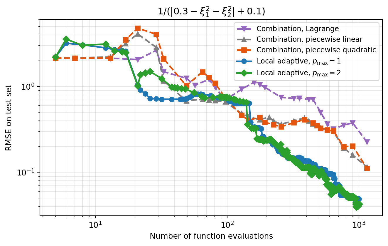
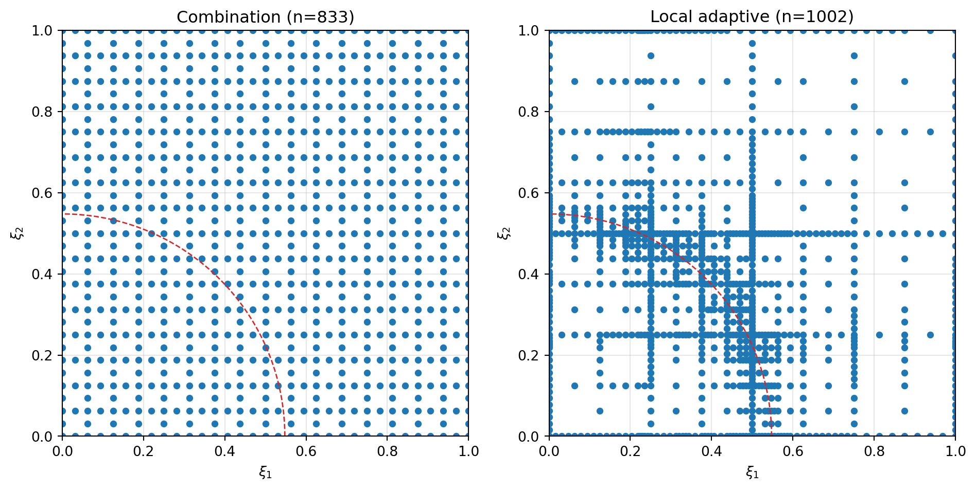
Point Distributions
The advantage is visible in the node placement: the combination technique refines whole axes uniformly, while local refinement clusters points along the ridge \(\xi_1^2 + \xi_2^2 = 0.3\).
Why Local Adaptivity Wins
The combination technique selects whole subspaces. When the indicator identifies a dimension as important it refines the entire axis to the next level — adding nodes uniformly even in smooth regions far from the ridge. Local adaptivity instead refines the single point with the largest surplus, so evaluations concentrate where the function is hardest to approximate.
Summary
| Method | Refines | Behavior on localized features | API |
|---|---|---|---|
| Combination, piecewise | Whole subspaces | Uniform refinement along important axes; wastes evaluations in smooth regions | SingleFidelityAdaptiveSparseGridFitter + PiecewiseFactory |
| Local adaptive (\(p_{\max}{=}1\)) | Single points | Concentrates evaluations on the feature | SingleFidelityHierarchicalFitter + HierarchicalBasis1D(p_max=1) |
| Local adaptive (\(p_{\max}{=}2\)) | Single points | Same concentration; higher accuracy in smooth regions | HierarchicalBasis1D(p_max=2) |
Exercises
- Set
downward_closed=Falseinrun_local. Does the convergence curve improve or degrade? Inspect the point distribution to explain. - Replace
target_fnwith a smooth function such as \(\cos(\pi \xi_1)\cos(\pi \xi_2/2)\). Does the local-vs-combination gap shrink, grow, or stay the same? - Reduce
max_ptsto 100. Is the gap between the two methods already visible at small budgets?