import numpy as np
np.random.seed(42)

from pyapprox.util.backends.numpy import NumpyBkd
from pyapprox.probability.univariate.beta import BetaMarginal
from pyapprox.probability.joint.independent import IndependentJoint

bkd = NumpyBkd()

# Beta marginals on +/- 10% of nominal values
E1_nom, E2_nom = 20_000, 5_000
beta_E1 = BetaMarginal(2.0, 6.0, bkd, lb=0.9 * E1_nom, ub=1.1 * E1_nom)
beta_E2 = BetaMarginal(6.0, 2.0, bkd, lb=0.9 * E2_nom, ub=1.1 * E2_nom)

# Independent joint distribution
variable_indep = IndependentJoint([beta_E1, beta_E2], bkd)

samples_indep = variable_indep.rvs(3000)Random Variables and Distributions
PyApprox Tutorial Library
Specifying parameter uncertainty with independent and copula-based distributions.
TipDownload Notebook
Learning Objectives
After completing this tutorial, you will be able to:
- Represent uncertain model parameters as random variables with specified distributions
- Construct an independent joint distribution from marginal distributions
- Use a copula to combine marginals with a prescribed correlation structure
- Sample from each type of distribution and visualize the resulting prior
Prerequisites
Complete Forward Uncertainty Quantification before this tutorial.
From Uncertainty to Probability Distributions
The opening tutorial showed that the beam’s material properties are uncertain, and the forward UQ tutorial showed that propagating that uncertainty requires a probability distribution over the uncertain parameters. But where does this distribution come from?
In practice, the choice of distribution encodes our state of knowledge about the parameters:
- A manufacturer’s data sheet might report \(E = 20{,}000 \pm 2{,}000\) — suggesting a distribution centered at \(20{,}000\) with some spread.
- Physical constraints might bound a parameter: a Young’s modulus must be positive, a Poisson ratio must lie in \([0, 0.5)\).
- We might know two parameters are correlated: if the skin and core come from the same batch of raw material, their stiffnesses tend to be high or low together.
This tutorial introduces two ways to specify the joint distribution of uncertain parameters, using the composite cantilever beam as the running example.
The Uncertain Parameters
We treat the beam as having two uncertain parameters:
| Symbol | Meaning | Nominal value |
|---|---|---|
| \(E_1\) | Young’s modulus of the outer skins (top and bottom layers) | \(20{,}000\) |
| \(E_2\) | Young’s modulus of the inner core | \(5{,}000\) |
The Poisson ratios (\(\nu_1 = \nu_2 = 0.3\)) and geometry are treated as fixed. The parameter vector is \(\params = (E_1, E_2)\).
Why Not Gaussian?
A Gaussian distribution is unbounded: it assigns nonzero probability to negative values and to arbitrarily large values. For a Young’s modulus, which must be positive and has a physically plausible range, a bounded distribution is more appropriate.
A Beta distribution is defined on a finite interval and can represent symmetric or skewed uncertainty depending on its shape parameters \((\alpha, \beta)\). When \(\alpha \neq \beta\) the density is skewed: \(\alpha < \beta\) concentrates mass toward the lower bound, while \(\alpha > \beta\) concentrates it toward the upper bound. We set the interval to \(\pm 10\%\) of the nominal value so that every sample is physically admissible.
Independent Beta Marginals
The simplest specification: each parameter follows its own Beta distribution, and the two are independent — knowing the value of \(E_1\) tells us nothing about \(E_2\).
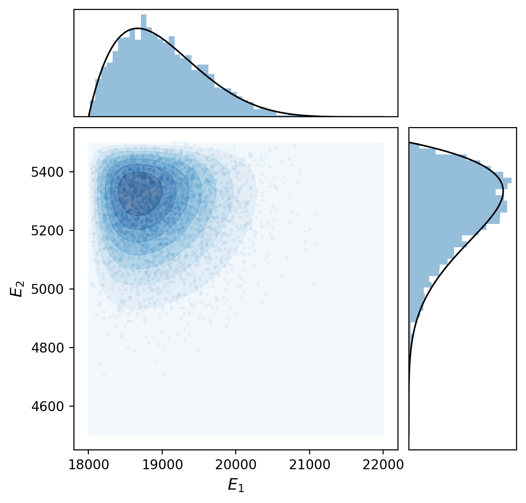
\[ E_1 \sim \text{Beta}(2, 6) \;\text{on}\; [18{,}000,\; 22{,}000], \qquad E_2 \sim \text{Beta}(6, 2) \;\text{on}\; [4{,}500,\; 5{,}500] \]
\[ \pdf(E_1, E_2) = \pdf_1(E_1) \cdot \pdf_2(E_2) \]
The joint density is the product of the marginals — this is the defining property of independence.
Figure 1 shows the joint distribution: a scatter plot of the samples with marginal histograms and contours of the joint PDF. Because the parameters are independent, the contours are axis-aligned — there is no preferred diagonal direction.
Introducing Correlation with a Copula
In many applications, uncertain parameters are not independent. For our beam, if the skin and core materials are produced by the same manufacturer or tested under similar conditions, high \(E_1\) and high \(E_2\) may tend to occur together. This is positive correlation.
We cannot simply construct a “multivariate Beta” — no standard one exists. Instead, a copula separates the marginal distributions from the dependence structure.
NoteWhat is a copula?
A copula separates the marginal distributions (the shape of each parameter’s individual distribution) from the dependence structure (how the parameters co-vary). The recipe is:
- Choose marginal distributions for each parameter (e.g., Beta for \(E_1\), Beta for \(E_2\)).
- Choose a copula family that describes the dependence (e.g., Gaussian copula with correlation \(\rho\)).
- The copula glues the marginals together into a valid joint distribution.
This allows us to combine any marginal distributions with any correlation pattern.
A Gaussian copula with correlation \(\rho\) works as follows:
- Draw correlated standard normals \((z_1, z_2)\) with correlation \(\rho\).
- Transform each to \([0, 1]\) via the standard normal CDF: \(u_i = \Phi(z_i)\).
- Apply each marginal’s inverse CDF: \(E_i = F_i^{-1}(u_i)\).
The result: samples that respect the Beta marginals and exhibit the desired correlation.
from pyapprox.probability.copula.bivariate.gaussian import (
    BivariateGaussianCopula,
)
from pyapprox.probability.copula.distribution import CopulaDistribution

# Gaussian copula with rho = 0.95
copula = BivariateGaussianCopula(rho=0.95, bkd=bkd)
variable_copula = CopulaDistribution(copula, [beta_E1, beta_E2], bkd)

samples_copula = variable_copula.sample(3000)
corr = np.corrcoef(bkd.to_numpy(samples_copula[0]),
                    bkd.to_numpy(samples_copula[1]))[0, 1]
print(f"Empirical correlation: {corr:.3f}")
Empirical correlation: 0.882Figure 2 shows the result. Compared to the independent case, the scatter cloud is now tilted: high \(E_1\) tends to occur with high \(E_2\).

Why Correlation Matters for UQ
Correlation changes the push-forward distribution. Consider two cases for the beam:
Positive correlation (\(\rho > 0\)): When \(E_1\) is low, \(E_2\) tends to be low too. The beam is uniformly compliant, and \(\delta_{\text{tip}}\) is large. The combination “stiff skin, soft core” (which might partially compensate) is unlikely. This concentrates extreme outcomes.
Independence (\(\rho = 0\)): All combinations of \(E_1\) and \(E_2\) within their ranges are equally possible (up to the marginal densities). The QoI distribution reflects the full range of parameter combinations.
Ignoring correlation when it exists leads to incorrect uncertainty estimates.
Comparing the Two Priors
Figure 3 compares the independent and copula-based joint distributions side by side. Each encodes a different set of assumptions about the uncertain parameters, and as the forward UQ tutorial showed, different input distributions produce different push-forward distributions — and therefore different engineering conclusions.
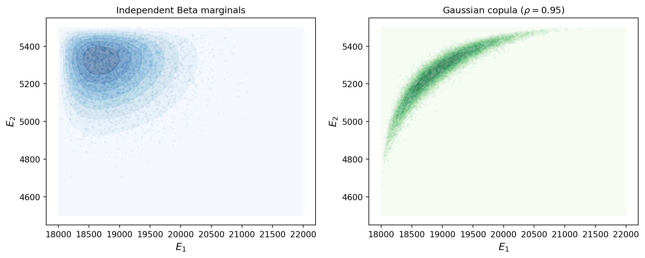
The choice between these specifications should be driven by the available data and physical knowledge:
- Use independent marginals when you have no evidence of correlation and want the simplest model.
- Use a copula with bounded marginals when you have evidence of dependence between parameters, or when physical constraints demand bounded support.
Higher Dimensions: Three Uncertain Parameters
Real problems typically have more than two uncertain parameters. Suppose we now also treat the Poisson ratio \(\nu\) as uncertain, giving three parameters:
| Symbol | Marginal | Range |
|---|---|---|
| \(E_1\) | Beta(2, 6) | \([18{,}000,\; 22{,}000]\) |
| \(E_2\) | Beta(6, 2) | \([4{,}500,\; 5{,}500]\) |
| \(\nu\) | Beta(3, 5) | \([0.25,\; 0.35]\) |
A multivariate Gaussian copula generalizes the bivariate case to any number of dimensions. Instead of a single correlation \(\rho\), we specify a full correlation matrix \(\mt{R}\):
\[ \mt{R} = \begin{pmatrix} 1 & 0.8 & 0.3 \\ 0.8 & 1 & 0.5 \\ 0.3 & 0.5 & 1 \end{pmatrix} \]
The copula draws correlated standard normals with this correlation structure, transforms them to \([0, 1]\) via the normal CDF, and applies each marginal’s inverse CDF — exactly as in the bivariate case.
from pyapprox.probability.copula.correlation.cholesky import (
    CholeskyCorrelationParameterization,
)
from pyapprox.probability.copula.gaussian import GaussianCopula

# Third marginal: Poisson ratio
beta_nu = BetaMarginal(3.0, 5.0, bkd, lb=0.25, ub=0.35)

# Correlation matrix
Sigma = np.array([[1.0, 0.8, 0.3],
                   [0.8, 1.0, 0.5],
                   [0.3, 0.5, 1.0]])

# Cholesky parameterization for the copula
L_chol = np.linalg.cholesky(Sigma)
chol_params = bkd.asarray(np.array([L_chol[1, 0], L_chol[2, 0], L_chol[2, 1]]))
corr_param = CholeskyCorrelationParameterization(chol_params, nvars=3, bkd=bkd)

copula_3d = GaussianCopula(corr_param, bkd)
variable_3d = CopulaDistribution(copula_3d, [beta_E1, beta_E2, beta_nu], bkd)

samples_3d = variable_3d.sample(3000)
print(f"Sample shape: {samples_3d.shape}")
print(f"Empirical correlation matrix:")
print(np.round(np.corrcoef(bkd.to_numpy(samples_3d)), 2))
Sample shape: (3, 3000)
Empirical correlation matrix:
[[1. 0.74 0.29]
[0.74 1. 0.49]
[0.29 0.49 1. ]]To visualize a 3D distribution, we plot all pairwise 2D marginals on the lower triangle and the 1D marginals on the diagonal. The PairPlotter automates this using a dimension reducer — here we use FunctionMarginalizer with Gauss-Legendre quadrature to integrate out variables from the joint PDF.
from pyapprox.surrogates.quadrature.tensor_product_factory import (
    TensorProductQuadratureFactory,
)

# Build a tensor product Gauss-Legendre quadrature factory
quad_factory = TensorProductQuadratureFactory(
    npoints_1d=[20, 20, 20],
    domain=variable_3d.domain(),
    bkd=bkd,
)
Figure 4 shows the corner plot for the 3-parameter copula distribution. The plotter() method accepts the quadrature factory and builds the pair plot automatically.
plotter_3d = variable_3d.plotter(
    quad_factory=quad_factory,
    variable_names=[r"$E_1$", r"$E_2$", r"$\nu$"],
)
fig, axes = plotter_3d.plot(npts_1d=51, contour_kwargs={"cmap": "Blues"})
plt.tight_layout()
plt.show()
The corner plot reveals the full dependence structure at a glance: the strong correlation between \(E_1\) and \(E_2\) (\(\rho = 0.8\)) is visible as elongated contours along the diagonal, while the weaker correlation between \(E_1\) and \(\nu\) (\(\rho = 0.3\)) produces more circular contours.
Key Takeaways
- Uncertain parameters are represented as random variables with probability distributions that encode our state of knowledge
- The joint distribution \(\pdf(\params)\) specifies both the marginal behavior of each parameter and their dependence structure
- Beta distributions are well-suited for material parameters because they are bounded — every sample is physically admissible
- Independent marginals are the simplest specification: the joint density is the product of the marginals
- Copulas decouple marginal shapes from the dependence structure, allowing bounded marginals with arbitrary correlation
- Correlation can significantly affect the push-forward — ignoring it when present leads to incorrect uncertainty estimates
Next Steps
Continue with:
- Monte Carlo Sampling — Propagating these distributions through the beam model
- Sensitivity Analysis — Determining which parameter drives output uncertainty