import numpy as np
np.random.seed(42)
import matplotlib.pyplot as plt

from pyapprox.util.backends.numpy import NumpyBkd
from pyapprox.surrogates.kernels import ExponentialKernel
from pyapprox.surrogates.kle import MeshKLE, DataDrivenKLE

bkd = NumpyBkd()
rng = np.random.default_rng(0)

# Shared setup
npts = 150
x = np.linspace(0, 2, npts)
mesh_coords = bkd.array(x[None, :])

# Trapezoid quadrature weights
dx = x[1] - x[0]
w = np.ones(npts) * dx; w[0] /= 2; w[-1] /= 2
quad_weights = bkd.array(w)KLE II: Kernel-Based vs Data-Driven KLE
PyApprox Tutorial Library
Compare MeshKLE (kernel-based) and DataDrivenKLE (SVD of samples) for computing the Karhunen-Loeve Expansion.
TipDownload Notebook
Learning Objectives
After completing this tutorial, you will be able to:
- Use
MeshKLEto compute a KLE from a covariance kernel and mesh coordinates - Use
DataDrivenKLEto compute a KLE from field sample data via SVD - Compare eigenvalues and eigenfunctions from both methods
- Understand when to use each approach and the effect of sample count and mesh resolution
- Reconstruct a field from its KLE projection
Building on the foundations from KLE I, this tutorial compares two strategies for computing the KLE:
MeshKLE |
DataDrivenKLE |
|
|---|---|---|
| Input | Covariance kernel function | Field sample data |
| Method | Weighted eigendecomposition of \(C\) | SVD of sample matrix |
| When to use | Known kernel, no existing data | Data exists, kernel unknown |
| Accuracy | Limited by mesh resolution | Limited by number of samples |
How MeshKLE works: weighted eigendecomposition
Given mesh coordinates and a kernel, MeshKLE assembles the \(N \times N\) covariance matrix \(C_{ij} = k(x_i, x_j)\) and solves the weighted eigenproblem \(W^{1/2} C W^{1/2} \hat\phi = \lambda \hat\phi\) where \(W = \mathrm{diag}(w_i)\) are quadrature weights.
from pyapprox_tutorials.figures._kle import plot_mesh_kle_overview

nterms = 5
ell = 0.5

kernel = ExponentialKernel(bkd.array([ell]), (0.01, 10.0), 1, bkd)
kle_mesh = MeshKLE(
    mesh_coords, kernel, sigma=1.0, nterms=nterms,
    quad_weights=quad_weights, bkd=bkd,
)

lam_mesh = bkd.to_numpy(kle_mesh.eigenvalues())
phi_mesh = bkd.to_numpy(kle_mesh.eigenvectors())
C = bkd.to_numpy(kernel(mesh_coords, mesh_coords))

fig, axes = plt.subplots(1, 3, figsize=(14, 4))
plot_mesh_kle_overview(x, C, phi_mesh, nterms, w, axes[0], axes[1], axes[2], fig=fig)
plt.tight_layout()
plt.show()
MeshKLE eigenfunctions. Right: the Gram matrix \(\Phi^T W \Phi\) verifying weighted orthonormality (should be the identity).
The eigenvectors are W-orthonormal: \(\Phi^T W \Phi = I\) (near-identity above).
How DataDrivenKLE works: SVD of samples
Given \(N_s\) field realizations stacked as columns, DataDrivenKLE computes the SVD: \(A = U \Sigma V^T\). The left singular vectors \(U\) are the empirical eigenfunctions; the eigenvalues are \(\lambda_k = \sigma_k^2 / (N_s - 1)\).
from pyapprox_tutorials.figures._kle import plot_data_driven_eigenfunctions

# Generate samples from the MeshKLE to use as "data"
N_samples_list = [50, 500, 5000]
max_Ns = max(N_samples_list)
Z_big = bkd.array(rng.standard_normal((nterms, max_Ns)))
field_samples_big = bkd.to_numpy(kle_mesh(Z_big))

phi_dd_list = []
for Ns in N_samples_list:
    samples = bkd.array(field_samples_big[:, :Ns])
    kle_dd = DataDrivenKLE(
        samples, nterms=nterms, quad_weights=quad_weights, bkd=bkd,
    )
    phi_dd_list.append(bkd.to_numpy(kle_dd.eigenvectors()))

fig, axes = plt.subplots(1, 3, figsize=(14, 4))
plot_data_driven_eigenfunctions(x, phi_mesh, phi_dd_list, N_samples_list, nterms, axes)
fig.suptitle("DataDrivenKLE eigenfunctions (solid) vs MeshKLE reference (dashed)",
             fontsize=12)
plt.tight_layout()
plt.show()
DataDrivenKLE eigenfunctions (solid) vs MeshKLE reference (dashed) for increasing sample counts \(N_s = 50, 500, 5000\). With few samples the empirical modes are noisy; by \(N_s = 5000\) they closely match the kernel-based reference.
With \(N_s = 50\) the data-driven modes are noisy; by \(N_s = 5000\) they match the analytical eigenfunctions closely.
Eigenvalue convergence with sample count
from pyapprox_tutorials.figures._kle import plot_eigenvalue_convergence

Ns_range = np.logspace(1.5, 4, 25, dtype=int)
errors = np.zeros((len(Ns_range), nterms))
max_Ns2 = int(max(Ns_range))
Z_max = bkd.array(rng.standard_normal((nterms, max_Ns2)))
samples_max = bkd.to_numpy(kle_mesh(Z_max))

for i, Ns in enumerate(Ns_range):
    kle_dd = DataDrivenKLE(
        bkd.array(samples_max[:, :Ns]), nterms=nterms,
        quad_weights=quad_weights, bkd=bkd,
    )
    lam_dd = bkd.to_numpy(kle_dd.eigenvalues())
    errors[i] = np.abs(lam_dd - lam_mesh) / lam_mesh

# Eigenvectors with and without quadrature weights
Ns = 500
samples_500 = bkd.array(field_samples_big[:, :Ns])
kle_dd_w = DataDrivenKLE(
    samples_500, nterms=nterms, quad_weights=quad_weights, bkd=bkd,
)
kle_dd_no_w = DataDrivenKLE(
    samples_500, nterms=nterms, bkd=bkd,
)
phi_dd_w = bkd.to_numpy(kle_dd_w.eigenvectors())
phi_dd_no_w = bkd.to_numpy(kle_dd_no_w.eigenvectors())

fig, axes = plt.subplots(1, 2, figsize=(12, 4))
plot_eigenvalue_convergence(
    x, Ns_range, errors, nterms, phi_mesh,
    phi_dd_w, phi_dd_no_w, axes[0], axes[1],
)
plt.tight_layout()
plt.show()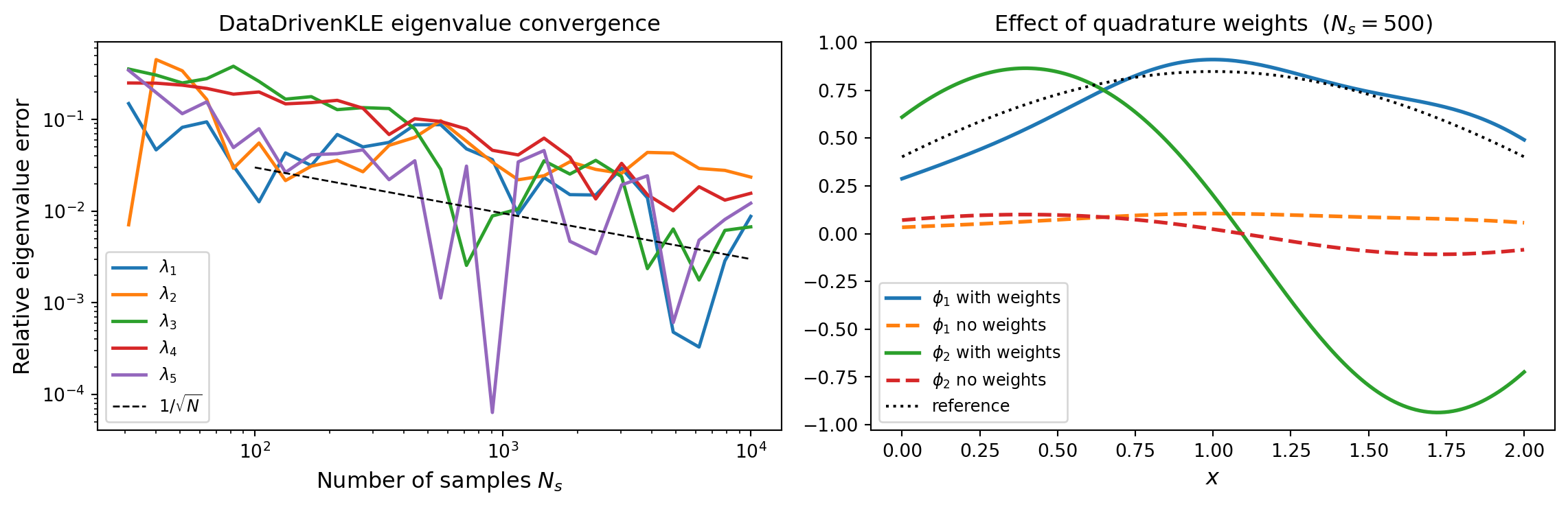
DataDrivenKLE vs sample count \(N_s\), decaying as \(1/\sqrt{N_s}\). Right: effect of quadrature weights on the first two eigenfunctions at \(N_s = 500\). Weights improve accuracy when the mesh spacing is non-uniform.
Key points: eigenvalue errors decay as \(1/\sqrt{N_s}\) (statistical estimation noise). Quadrature weights are important when the mesh is non-uniform – without them the SVD weights all nodes equally regardless of the cell size.
Mesh resolution: how fine does it need to be?
For MeshKLE, finer mesh yields a better approximation of the integral. The error in eigenvalue \(k\) scales as \(O(h^2)\) for the trapezoid rule.
from pyapprox.surrogates.kle import AnalyticalExponentialKLE1D
from pyapprox_tutorials.figures._kle import plot_mesh_convergence

npts_list = [20, 40, 80, 160, 320]

# Use analytical eigenvalues as reference (not the finest mesh)
kle_exact = AnalyticalExponentialKLE1D(
    corr_len=ell, sigma2=1.0, dom_len=2.0, nterms=nterms,
)
lam_ref = np.array(kle_exact.eigenvalues())

eig_errors_mesh = np.zeros((len(npts_list), nterms))
for i, npts_i in enumerate(npts_list):
    xi = np.linspace(0, 2, npts_i)
    dxi = xi[1] - xi[0]
    wi = np.ones(npts_i) * dxi; wi[0] /= 2; wi[-1] /= 2
    kernel_i = ExponentialKernel(bkd.array([ell]), (0.01, 10.0), 1, bkd)
    kle_i = MeshKLE(
        bkd.array(xi[None, :]), kernel_i, sigma=1.0, nterms=nterms,
        quad_weights=bkd.array(wi), bkd=bkd,
    )
    eig_errors_mesh[i] = bkd.to_numpy(kle_i.eigenvalues())

eig_errors_rel = np.abs(eig_errors_mesh - lam_ref) / lam_ref

table_data = [
    ["", "MeshKLE", "DataDrivenKLE"],
    ["Input required", "Kernel function", "Field samples"],
    ["Memory", "$O(N^2)$ dense", "$O(N \\cdot N_s)$"],
    ["Main error source", "Quadrature $O(h^2)$", "Stats $O(1/\\sqrt{N_s})$"],
    ["Extrapolate beyond data?", "Yes \u2014 any $x$", "Only on training mesh"],
    ["Unknown kernel?", "No", "Yes"],
]

fig, axes = plt.subplots(1, 2, figsize=(12, 4))
plot_mesh_convergence(npts_list, eig_errors_rel, nterms, table_data, axes[0], axes[1])
plt.tight_layout()
plt.show()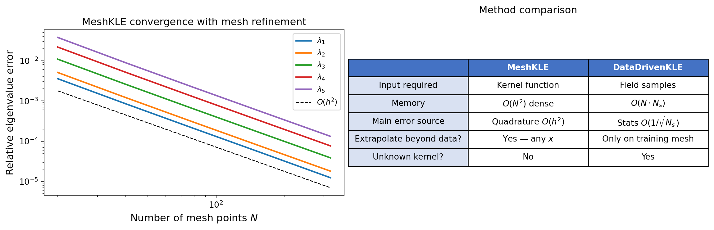
MeshKLE eigenvalue convergence with mesh refinement (relative to the analytical solution), showing \(O(h^2)\) convergence for the trapezoid rule. Right: summary comparison of MeshKLE vs DataDrivenKLE properties.
Reconstructing a field from new data
Both KLEs can project new observations onto the KLE basis. Given a field \(f(x)\), the projection coefficients are \(c_k = \langle f, \phi_k \rangle_w = \sum_i w_i\, f(x_i)\, \phi_k(x_i)\). The reconstruction with \(K\) terms is \(\hat{f}(x) = \sum_{k=1}^K c_k\, \sqrt{\lambda_k}\, \phi_k(x)\).
from pyapprox_tutorials.figures._kle import plot_field_reconstruction

# Generate a "new" realization for reconstruction
z_new = bkd.array(rng.standard_normal((nterms, 1)))
f_true = bkd.to_numpy(kle_mesh(z_new))[:, 0]

# Reconstruct using increasing number of terms
K_list = [1, 3, 5]
reconstructions = []
for K in K_list:
    kle_K = MeshKLE(
        mesh_coords, kernel, sigma=1.0, nterms=K,
        quad_weights=quad_weights, bkd=bkd,
    )
    phi_K = bkd.to_numpy(kle_K.eigenvectors())
    coeffs = (phi_K * w[:, None]).T @ f_true
    reconstructions.append(phi_K @ coeffs)

fig, axes = plt.subplots(1, 3, figsize=(14, 4))
plot_field_reconstruction(x, f_true, K_list, reconstructions, axes)
fig.suptitle("Field reconstruction from KLE projection", fontsize=12)
plt.tight_layout()
plt.show()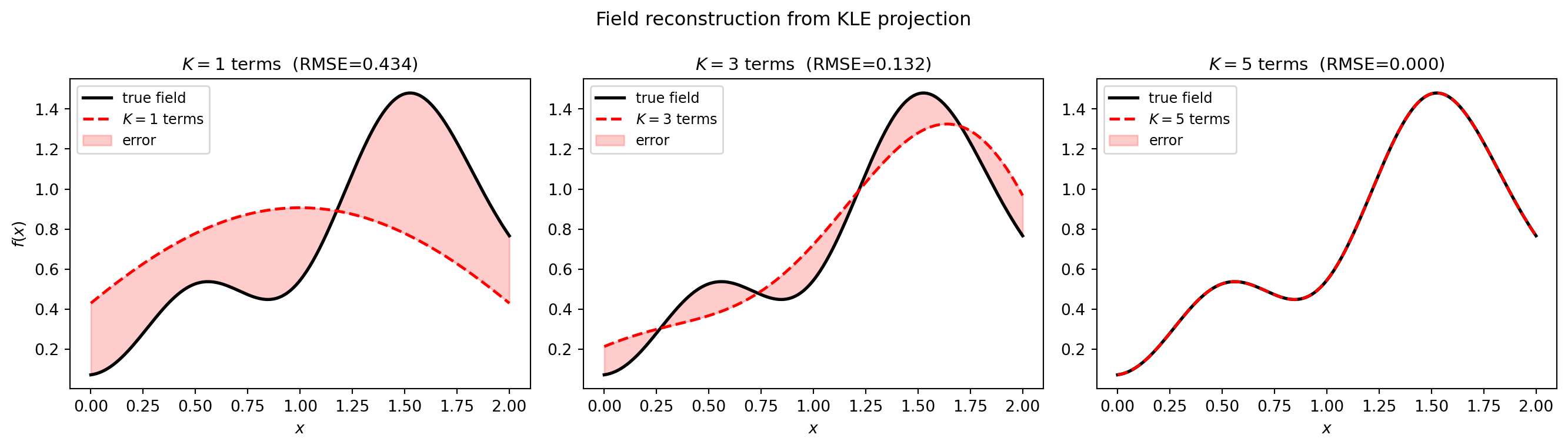
The reconstruction error decreases as \(K\) increases, driven by the eigenvalue spectrum – modes with small \(\lambda_k\) contribute little.
Summary: use MeshKLE when you have a kernel and want maximum accuracy with a fixed mesh; use DataDrivenKLE when you have sample data and either the kernel is unknown or you want to match the empirical covariance exactly. Next: KLE III covers SPDEMaternKLE, which replaces the dense \(C\) matrix with a sparse PDE operator to scale to large meshes.