---
title: "Sobol Sensitivity Analysis"
subtitle: "PyApprox Tutorial Library"
description: "Variance-based sensitivity indices for identifying important parameters"
tutorial_type: usage
topic: sensitivity_analysis
difficulty: intermediate
estimated_time: 10
render_time: 48
prerequisites:
- sensitivity_analysis_concept
tags:
- sensitivity-analysis
- sobol-indices
- monte-carlo
format:
html:
code-fold: false
code-tools: true
toc: true
execute:
echo: true
warning: false
jupyter: python3
---
::: {.callout-tip collapse="true"}
## Download Notebook
[Download as Jupyter Notebook](notebooks/sobol_sensitivity_analysis.ipynb)
:::
## Learning Objectives
After completing this tutorial, you will be able to:
- Explain variance-based sensitivity analysis
- Interpret first-order and total-order Sobol indices
- Estimate sensitivity indices using Monte Carlo
- Identify the most important parameters in a model
## Prerequisites
Complete [Sensitivity Analysis](sensitivity_analysis_concept.qmd) before this tutorial.
## Why Sensitivity Analysis?
**Sensitivity Analysis (SA)** answers: *Which parameters matter most?*
This helps us:
- **Focus resources** on reducing important uncertainties
- **Simplify models** by fixing unimportant parameters
- **Understand** model behavior and interactions
## Variance-Based Sensitivity
The idea: decompose output variance into contributions from each parameter.
Total variance:
$$
\Var_{\params}[q] = \Var_{\theta_1}[\E_{\theta_{\sim 1}}[q | \theta_1]] + \E_{\theta_1}[\Var_{\theta_{\sim 1}}[q | \theta_1]]
$$
The first term measures how much knowing $\theta_1$ reduces variance.
## Sobol Indices
### First-Order Index
The **first-order Sobol index** $\Sobol{i}$ measures the fraction of variance explained by parameter $\theta_i$ alone:
$$
\Sobol{i} = \frac{\Var_{\theta_i}[\E_{\theta_{\sim i}}[q | \theta_i]]}{\Var_{\params}[q]}
$$
- $\Sobol{i} \approx 1$: Parameter $i$ explains nearly all variance
- $\Sobol{i} \approx 0$: Parameter $i$ has little direct effect
### Total-Order Index
The **total-order Sobol index** $\SobolT{i}$ includes interactions with other parameters:
$$
\SobolT{i} = 1 - \frac{\Var_{\theta_{\sim i}}[\E_{\theta_i}[q | \theta_{\sim i}]]}{\Var_{\params}[q]}
$$
where $\theta_{\sim i}$ means all parameters except $\theta_i$.
- $\SobolT{i}$ includes direct effects AND interactions
- Always $\SobolT{i} \geq \Sobol{i}$
- If $\SobolT{i} \approx \Sobol{i}$: few interactions involving $\theta_i$
## Setup
```{python}
import numpy as np
import matplotlib.pyplot as plt
from pyapprox.util.backends.numpy import NumpyBkd
from pyapprox_benchmarks.ode import build_lotka_volterra_3species

bkd = NumpyBkd()
problem = build_lotka_volterra_3species(bkd)

# QoI: Species 1 final population
qoi_func = problem.function(functional="endpoint_0")
print(f"Model has {qoi_func.nvars()} parameters")
```
## Estimating Sobol Indices
We'll use a simple Monte Carlo approach. For a more efficient implementation, see PyApprox's built-in Sobol estimators.
### Generate Sample Matrices
The Sobol method requires two independent sample matrices:
```{python}
np.random.seed(42)

N = 1000  # Base sample size
d = 12    # Number of parameters
lower, upper = 0.3, 0.7

# Two independent sample matrices
A = lower + (upper - lower) * np.random.rand(d, N)
B = lower + (upper - lower) * np.random.rand(d, N)

print(f"Matrix A shape: {A.shape}")
print(f"Matrix B shape: {B.shape}")
```
### Evaluate Base Cases
```{python}
# Evaluate f(A) and f(B)
f_A = bkd.to_numpy(qoi_func(bkd.asarray(A))).flatten()
f_B = bkd.to_numpy(qoi_func(bkd.asarray(B))).flatten()

print(f"f(A) mean: {np.mean(f_A):.4f}")
print(f"f(B) mean: {np.mean(f_B):.4f}")
```
### Create Mixed Matrices
For each parameter $i$, create a matrix $C_i$ that equals $B$ except column $i$ comes from $A$:
```{python}
def make_C_matrix(A, B, i):
    """Create C_i matrix: B with column i from A."""
    C = B.copy()
    C[i, :] = A[i, :]
    return C

# Example: C_0 has parameter 0 from A, all others from B
C_0 = make_C_matrix(A, B, 0)
print(f"C_0 differs from B only in row 0:")
print(f"  B[0, :5] = {B[0, :5]}")
print(f"  C_0[0, :5] = {C_0[0, :5]}")
print(f"  A[0, :5] = {A[0, :5]}")
```
### Compute First-Order Indices
```{python}
# Estimate variance
var_total = np.var(np.concatenate([f_A, f_B]))

first_order = np.zeros(d)
for i in range(d):
    C_i = make_C_matrix(A, B, i)
    f_C_i = bkd.to_numpy(qoi_func(bkd.asarray(C_i))).flatten()

    # Jansen estimator for first-order index
    first_order[i] = np.mean(f_B * (f_C_i - f_A)) / var_total

print("First-order Sobol indices (S_i):")
for i, s in enumerate(first_order):
    print(f"  θ_{i:2d}: {s:.4f}")
```
### Compute Total-Order Indices
```{python}
total_order = np.zeros(d)
for i in range(d):
    C_i = make_C_matrix(A, B, i)
    f_C_i = bkd.to_numpy(qoi_func(bkd.asarray(C_i))).flatten()

    # Jansen estimator for total-order index
    total_order[i] = 0.5 * np.mean((f_A - f_C_i)**2) / var_total

print("Total-order Sobol indices (S^T_i):")
for i, st in enumerate(total_order):
    print(f"  θ_{i:2d}: {st:.4f}")
```
## Visualizing Results
```{python}
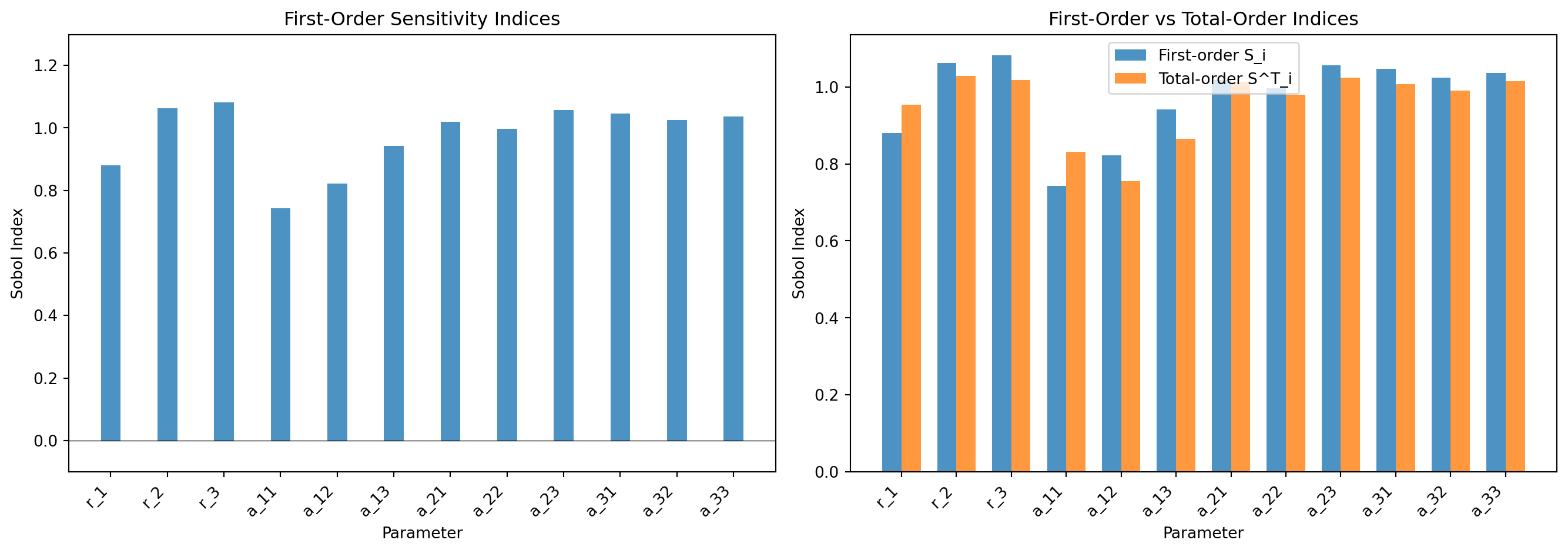
#| fig-cap: "Sobol index estimates for the 3-species Lotka--Volterra model (QoI: species 1 final population). Left: first-order indices $S_i$ showing direct parameter contributions. Right: comparison of first-order and total-order indices---large gaps (e.g. interaction coefficients) indicate parameter interactions."
#| label: fig-sobol-indices
from pyapprox_tutorials.figures._sensitivity import plot_sobol_indices

# Parameter labels
labels = [f'r_{i}' for i in range(1, 4)] + \
         [f'a_{i//3+1}{i%3+1}' for i in range(9)]

fig, axes = plt.subplots(1, 2, figsize=(14, 5))
plot_sobol_indices(first_order, total_order, labels, d, axes)
plt.tight_layout()
plt.show()
```
## Interpreting Results
```{python}
# Sort parameters by total-order importance
importance_order = np.argsort(total_order)[::-1]

print("Parameters ranked by importance (total-order):")
print("-" * 50)
print(f"{'Rank':<6}{'Param':<8}{'S_i':<10}{'S^T_i':<10}{'Interaction':<12}")
print("-" * 50)

for rank, i in enumerate(importance_order[:6]):  # Top 6
    interaction = total_order[i] - first_order[i]
    print(f"{rank+1:<6}{labels[i]:<8}{first_order[i]:<10.4f}{total_order[i]:<10.4f}{interaction:<12.4f}")
```
### Key Observations
```{python}
# Sum of first-order indices
sum_first = np.sum(first_order)
print(f"\nSum of first-order indices: {sum_first:.4f}")

# If sum ≈ 1, model is mostly additive (few interactions)
# If sum << 1, strong interactions exist

if sum_first > 0.9:
    print("  → Model is approximately additive (few interactions)")
elif sum_first > 0.7:
    print("  → Moderate interactions present")
else:
    print("  → Strong parameter interactions")
```
## Sensitivity by Parameter Group
Let's aggregate sensitivity by parameter type:
```{python}
# Group indices
growth_rates = [0, 1, 2]  # r_1, r_2, r_3
competition_diag = [3, 6, 9]  # a_11, a_22, a_33 (self-competition)
competition_off = [4, 5, 7, 8, 10, 11]  # off-diagonal (inter-species)

group_sensitivity = {
    'Growth rates': np.sum(total_order[growth_rates]),
    'Self-competition': np.sum(total_order[competition_diag]),
    'Inter-competition': np.sum(total_order[competition_off]),
}

print("Aggregated sensitivity by parameter group:")
for group, sens in group_sensitivity.items():
    print(f"  {group}: {sens:.4f}")
```
```{python}
#| fig-cap: "Total-order sensitivity aggregated by parameter group. Growth rates ($r_i$) and self-competition ($a_{ii}$) dominate; inter-species competition ($a_{ij}, i \\neq j$) contributes the remainder."
#| label: fig-group-pie
from pyapprox_tutorials.figures._sensitivity import plot_group_pie

fig, ax = plt.subplots(figsize=(8, 6))
plot_group_pie(group_sensitivity, ax)
plt.show()
```
## Practical Implications
Based on the sensitivity analysis:
```{python}
# Find unimportant parameters (S^T < 0.01)
unimportant = np.where(total_order < 0.01)[0]
print(f"\nParameters with negligible influence (S^T < 0.01):")
if len(unimportant) > 0:
    for i in unimportant:
        print(f"  {labels[i]}: S^T = {total_order[i]:.4f}")
else:
    print("  None (all parameters are somewhat important)")

# Find dominant parameters (S_i > 0.1)
dominant = np.where(first_order > 0.1)[0]
print(f"\nDominant parameters (S_i > 0.1):")
if len(dominant) > 0:
    for i in dominant:
        print(f"  {labels[i]}: S_i = {first_order[i]:.4f}")
else:
    print("  None (no single parameter dominates)")
```
## Summary of Sobol Indices
| Index | Formula | Interpretation |
|-------|---------|----------------|
| $\Sobol{i}$ | $\frac{\Var_{\theta_i}[\E_{\theta_{\sim i}}[q|\theta_i]]}{\Var_{\params}[q]}$ | Direct effect of $\theta_i$ alone |
| $\SobolT{i}$ | $1 - \frac{\Var_{\theta_{\sim i}}[\E_{\theta_i}[q|\theta_{\sim i}]]}{\Var_{\params}[q]}$ | Total effect including interactions |
| $\SobolT{i} - \Sobol{i}$ | - | Interaction effects involving $\theta_i$ |
## Key Takeaways
- **Sobol indices** decompose variance by parameter contribution
- **First-order** $\Sobol{i}$: direct effect of parameter $i$
- **Total-order** $\SobolT{i}$: total effect including interactions
- **Sum of $\Sobol{i}$** indicates how additive the model is
- Focus uncertainty reduction on **high $\SobolT{i}$** parameters
## Exercises
1. **(Easy)** Compute Sobol indices for Species 2 final population. How do the important parameters differ from Species 1?
2. **(Medium)** Create a convergence plot showing how the Sobol index estimates for the top 3 parameters stabilize as N increases from 100 to 2000.
3. **(Challenge)** Compute Sobol indices for the "max" QoI functional (maximum population over time). Compare to the endpoint indices. What changes in the importance ranking?
## Next Steps
Continue with:
- [Bin-Based Sensitivity](bin_based_sensitivity.qmd) --- Sensitivity indices from existing datasets via binning
- [PCE-Based Sensitivity](pce_sensitivity.qmd) --- Sobol indices from polynomial chaos surrogates