import numpy as np
import matplotlib.pyplot as plt

from pyapprox.util.backends.numpy import NumpyBkd
from pyapprox.surrogates.sparsegrids import (
    IsotropicSparseGridFitter,
    SingleFidelityAdaptiveSparseGridFitter,
    TensorProductSubspaceFactory,
)
from pyapprox.surrogates.sparsegrids.basis_factory import (
    ClenshawCurtisLagrangeFactory,
)
from pyapprox.surrogates.affine.indices import (
    ClenshawCurtisGrowthRule,
    MaxLevelCriteria,
    Max1DLevelsCriteria,
    CompositeCriteria,
)
from pyapprox.probability.univariate.uniform import UniformMarginal
from pyapprox.interface.functions.plot.plot2d_rectangular import (
    Plotter2DRectangularDomain,
)
from pyapprox.interface.functions.fromcallable.function import (
    FunctionFromCallable,
)
from pyapprox_tutorials.figures._quadrature import (
    plot_additive_function,
    plot_index_set,
    plot_points_compare,
    plot_adaptive_vs_iso,
    plot_4d_adaptive,
)

bkd = NumpyBkd()
np.random.seed(42)Adaptive Sparse Grids: Data-Driven Refinement for Anisotropic Functions
PyApprox Tutorial Library
Implement the greedy adaptive algorithm, configure admissibility criteria, visualize index set evolution, and compare adaptive vs. isotropic sparse grids on anisotropic functions.
TipDownload Notebook
Learning Objectives
After completing this tutorial, you will be able to:
- Explain why adaptive refinement outperforms isotropic grids for anisotropic functions
- Use the
step_samples()/step_values()pattern withSingleFidelityAdaptiveSparseGridFitter - Understand the knapsack formulation of index set selection
- Configure admissibility criteria:
MaxLevelCriteria,Max1DLevelsCriteria,CompositeCriteria - Visualise the adaptive refinement process: index sets, point distributions, and convergence
- Compare adaptive vs. isotropic convergence on anisotropic and 4D benchmark functions
Prerequisites
Complete Isotropic Sparse Grids before this tutorial. You should understand the Smolyak combination technique, downward-closed index sets, and the IsotropicSparseGridFitter API.
Setup
Motivation: Anisotropy
The isotropic sparse grid treats all dimensions symmetrically: level \(l\) in dimension 1 pairs with level \(l\) in dimension 2. For anisotropic functions — where variation is concentrated in a subset of dimensions — this symmetry is wasteful. An adaptive algorithm that allocates more nodes to the high-variation dimensions and fewer to the low-variation ones will reach a given error tolerance with far fewer function evaluations.
Consider \(f(z_1, z_2) = \cos(5z_1) + 0.1 z_2\). This function varies much more in \(z_1\) than in \(z_2\). The isotropic grid places equal resources in both dimensions; an adaptive grid should concentrate almost all nodes along the \(z_1\) axis.
def additive_function(samples, bkd):
    """f(z1, z2) = cos(5*z1) + 0.1*z2. Shape: (1, nsamples)."""
    z1, z2 = samples[0, :], samples[1, :]
    values = bkd.cos(5.0 * z1) + 0.1 * z2
    return bkd.reshape(values, (1, -1))

func_2d = FunctionFromCallable(
    nqoi=1, nvars=2,
    fun=lambda s: additive_function(s, bkd),
    bkd=bkd,
)

fig, ax = plt.subplots(figsize=(7, 5))
plotter = Plotter2DRectangularDomain(func_2d, [-1, 1, -1, 1])
plot_additive_function(ax, plotter)
plt.tight_layout()
plt.show()
The Adaptive Algorithm
Finding the optimal downward-closed index set can be cast as a binary knapsack problem. Let \(\Delta E_\beta\) and \(\Delta W_\beta\) be the reduction in approximation error and the computational cost, respectively, of adding sub-grid \(\beta\):
\[ \max_{\delta} \sum_{\beta} \Delta E_\beta\, \delta_\beta \quad \text{subject to} \quad \sum_{\beta} \Delta W_\beta\, \delta_\beta \leq W_{\max}, \quad \delta_\beta \in \{0, 1\}. \]
Solving this exactly is intractable, so PyApprox uses a greedy adaptive procedure:
- Begin with \(\mathcal{I} = \{\mathbf{0}\}\).
- Identify active indices — candidates satisfying downward closure that are not yet in \(\mathcal{I}\).
- Evaluate \(f\) at all points associated with active indices.
- Compute an error indicator \(\Delta E_\beta\) for each active index (e.g., variance of the sub-space contribution).
- Add the active index with the largest indicator to \(\mathcal{I}\).
- Update the active set. Repeat until the budget is exhausted.
The Step Pattern
SingleFidelityAdaptiveSparseGridFitter uses a step pattern for incremental construction:
while True:
    new_samples = fitter.step_samples()  # Get new sample points
    if new_samples is None:
        break  # All admissible indices exhausted
    new_values = my_function(new_samples)
    fitter.step_values(new_values)        # Provide function values
Each call to step_samples() returns the points for the next candidate subspace. After evaluating the function at those points and passing the values back via step_values(), the algorithm decides which subspace to add based on the error indicator.
nvars = 2
marginal = UniformMarginal(-1.0, 1.0, bkd)
factories = [ClenshawCurtisLagrangeFactory(marginal, bkd) for _ in range(nvars)]
growth = ClenshawCurtisGrowthRule()

# Admissibility: maximum total level (set high so it does not activate)
admissibility = MaxLevelCriteria(max_level=20, pnorm=1.0, bkd=bkd)

# Create adaptive sparse grid fitter
tp_factory = TensorProductSubspaceFactory(bkd, factories, growth)
fitter = SingleFidelityAdaptiveSparseGridFitter(bkd, tp_factory, admissibility)

# Test samples for error estimation
n_test = 2000
test_samples = bkd.asarray(np.random.uniform(-1, 1, (nvars, n_test)))
true_values = additive_function(test_samples, bkd)

# Track convergence --- stop when error estimate drops below tolerance
nsamples_history = []
error_history = []
tol = 1e-12

for step in range(100):
    new_samples = fitter.step_samples()
    if new_samples is None:
        break

    new_values = additive_function(new_samples, bkd)
    fitter.step_values(new_values)

    # Track approximation error on test set
    ada_result = fitter.result()
    if ada_result.nsamples > 1:
        approx_values = ada_result.surrogate(test_samples)
        error = float(
            bkd.sqrt(bkd.sum((true_values - approx_values) ** 2))
            / np.sqrt(n_test)
        )
        nsamples_history.append(ada_result.nsamples)
        error_history.append(error)

    # Stop when the fitter's built-in error estimate is small
    if fitter.current_error() < tol:
        break

ada_result = fitter.result()
fig, ax = plt.subplots(figsize=(8, 5))
ax.semilogy(nsamples_history, error_history, "o-", color="#2C7FB8", lw=2, ms=5)
ax.set_xlabel("Number of samples", fontsize=12)
ax.set_ylabel("RMS Error", fontsize=12)
ax.set_title("Adaptive Sparse Grid Convergence", fontsize=12)
ax.grid(True, which="both", alpha=0.3)
plt.tight_layout()
plt.show()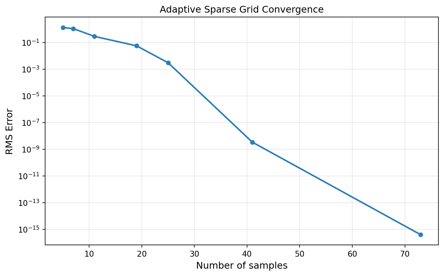
Visualizing the Selected Index Set
Because \(f\) is additive (\(f = g_1(z_1) + g_2(z_2)\)), no mixed terms are needed: the ideal index set consists only of axis-aligned indices \((k, 0)\) and \((0, k)\). The adaptive algorithm discovers both the additive structure (no cross-indices) and the anisotropy (more levels in \(z_1\) than \(z_2\)):
selected = ada_result.indices
sel_np = bkd.to_numpy(selected).astype(int)

fig, ax = plt.subplots(figsize=(8, 6))
plot_index_set(ax, sel_np)
plt.tight_layout()
plt.show()
Notice that the index set contains only axis-aligned indices — no cross-terms like \((2, 1)\) or \((1, 2)\) — reflecting the additive structure of \(f\). It also extends much further in \(k_1\) than in \(k_2\), reflecting the much stronger dependence on \(z_1\).
Visualizing Grid Points
# Adaptive points --- selected vs candidate
ada_selected = bkd.to_numpy(fitter.get_samples("selected"))
ada_candidate = bkd.to_numpy(fitter.get_samples("candidate"))

# Isotropic with comparable point count
iso_level = 4
iso_tp_factory = TensorProductSubspaceFactory(bkd, factories, growth)
iso_fitter = IsotropicSparseGridFitter(bkd, iso_tp_factory, iso_level)
iso_samples = bkd.to_numpy(iso_fitter.get_samples())
iso_nsamples = iso_samples.shape[1]

fig, axes = plt.subplots(1, 2, figsize=(12, 5))
plot_points_compare(
    axes, ada_selected, ada_candidate, ada_result.nsamples,
    iso_samples, iso_nsamples, iso_level,
)
plt.tight_layout()
plt.show()
Convergence Comparison: Adaptive vs. Isotropic
# Isotropic convergence
iso_nsamples_list, iso_errors = [], []

for level in range(7):
    iso_tp_fac = TensorProductSubspaceFactory(bkd, factories, growth)
    iso_fit = IsotropicSparseGridFitter(bkd, iso_tp_fac, level)
    iso_samp = iso_fit.get_samples()
    iso_vals = additive_function(iso_samp, bkd)
    iso_res = iso_fit.fit(iso_vals)

    approx = iso_res.surrogate(test_samples)
    error = float(
        bkd.sqrt(bkd.sum((true_values - approx) ** 2)) / np.sqrt(n_test)
    )
    iso_nsamples_list.append(iso_samp.shape[1])
    iso_errors.append(error)

fig, ax = plt.subplots(figsize=(8, 5))
plot_adaptive_vs_iso(ax, nsamples_history, error_history,
                     iso_nsamples_list, iso_errors)
plt.tight_layout()
plt.show()
Admissibility Criteria
The admissibility criteria determine which indices are allowed as candidates for refinement.
| Criterion | Constraint | Use case |
|---|---|---|
MaxLevelCriteria(l, pnorm) |
\(\lVert\beta\rVert_p \leq l\) | Total budget |
Max1DLevelsCriteria(max_levels) |
\(\beta_i \leq l_i\) for all \(i\) | Per-dimension cap |
CompositeCriteria(c1, c2) |
\(c_1(\beta) \wedge c_2(\beta)\) | AND of multiple criteria |
# Per-dimension maximum levels: more refinement in z1 than z2
max_levels = bkd.asarray([8, 4])
per_dim = Max1DLevelsCriteria(max_levels, bkd=bkd)

# Combine with total level budget
combined = CompositeCriteria(
    MaxLevelCriteria(max_level=10, pnorm=1.0, bkd=bkd),
    per_dim,
)

# Build adaptive grid with combined criteria
custom_tp_factory = TensorProductSubspaceFactory(bkd, factories, growth)
custom_fitter = SingleFidelityAdaptiveSparseGridFitter(
    bkd, custom_tp_factory, combined,
)

for _ in range(25):
    s = custom_fitter.step_samples()
    if s is None:
        break
    custom_fitter.step_values(additive_function(s, bkd))
    if custom_fitter.current_error() < 1e-12:
        break

custom_result = custom_fitter.result()
4D Adaptive Example
Adaptive refinement pays larger dividends in higher dimensions, especially when the function depends strongly on only a few inputs.
nvars4 = 4

def fun4d_additive(samples, bkd):
    """sin(3*z1) + 0.5*z2 + 0.1*z3 + 0.1*z4. Shape: (1, nsamples)."""
    z1, z2, z3, z4 = samples[0], samples[1], samples[2], samples[3]
    values = bkd.sin(3 * z1) + 0.5 * z2 + 0.1 * z3 + 0.1 * z4
    return bkd.reshape(values, (1, -1))

facs_4d = [ClenshawCurtisLagrangeFactory(marginal, bkd) for _ in range(nvars4)]

# Test samples
test_4d = bkd.asarray(np.random.uniform(-1, 1, (nvars4, 2000)))
true_4d = fun4d_additive(test_4d, bkd)

# Adaptive grid with error-based stopping
adm_4d = MaxLevelCriteria(max_level=20, pnorm=1.0, bkd=bkd)
tp_fac_4d = TensorProductSubspaceFactory(bkd, facs_4d, growth)
adaptive_4d = SingleFidelityAdaptiveSparseGridFitter(bkd, tp_fac_4d, adm_4d)

adapt_nsamples, adapt_errors = [], []
for step in range(100):
    s = adaptive_4d.step_samples()
    if s is None:
        break
    adaptive_4d.step_values(fun4d_additive(s, bkd))
    r4 = adaptive_4d.result()
    if r4.nsamples > 1:
        approx = r4.surrogate(test_4d)
        err = float(
            bkd.sqrt(bkd.sum((true_4d - approx) ** 2)) / np.sqrt(2000)
        )
        adapt_nsamples.append(r4.nsamples)
        adapt_errors.append(err)
    if adaptive_4d.current_error() < 1e-12:
        break

# Isotropic comparison
iso_nsamples_4d, iso_errors_4d = [], []
for level in range(5):
    iso_tp_fac4 = TensorProductSubspaceFactory(bkd, facs_4d, growth)
    iso_fit4 = IsotropicSparseGridFitter(bkd, iso_tp_fac4, level)
    iso_samp4 = iso_fit4.get_samples()
    iso_res4 = iso_fit4.fit(fun4d_additive(iso_samp4, bkd))
    approx = iso_res4.surrogate(test_4d)
    err = float(
        bkd.sqrt(bkd.sum((true_4d - approx) ** 2)) / np.sqrt(2000)
    )
    iso_nsamples_4d.append(iso_samp4.shape[1])
    iso_errors_4d.append(err)

fig, ax = plt.subplots(figsize=(8, 5))
plot_4d_adaptive(ax, adapt_nsamples, adapt_errors,
                 iso_nsamples_4d, iso_errors_4d)
plt.tight_layout()
plt.show()
Summary
- Adaptive sparse grids discover the structure of \(f\) from function evaluations alone: for additive functions the algorithm selects only axis-aligned indices (no cross-terms), and for anisotropic functions it allocates more levels to the important dimensions.
- The greedy adaptive algorithm selects the index with the largest variance indicator at each step, approximating the solution to a knapsack optimization problem.
- For strongly anisotropic functions, adaptive grids can achieve the same accuracy as isotropic grids at a fraction of the cost — the advantage grows with the degree of anisotropy.
- Admissibility criteria (
MaxLevelCriteria,Max1DLevelsCriteria,CompositeCriteria) provide flexible budget and safety constraints on the index set. - The step-based API (
step_samples()/step_values()) allows fine-grained control; usefitter.current_error()to stop when the estimated error drops below a tolerance. - For UQ with sparse grids (moments, Sobol indices, marginal densities), see UQ with Sparse Grids.
Exercises
NoteExercises
Anisotropy detection. Run the adaptive algorithm on \(f(z_1, z_2, z_3) = \cos(4z_1) + 0.1 z_2 + 0.01 z_3\). After convergence, visualize the index set. Does the algorithm correctly rank dimensions by importance?
Budget comparison. For the 2D additive benchmark, compare adaptive and isotropic grids at 50, 100, and 200 evaluations. At what budget does adaptive become clearly superior?
Criteria impact. Build an adaptive grid with
Max1DLevelsCriterialimiting \(z_2\) to level 2. Compare the resulting index set and convergence to the unconstrained case.Statistics. For the 2D benchmark, track \(\mathbb{E}[f]\) at each step of the adaptive algorithm and plot its convergence to the analytical value \(\sin(5)/5\). Compare with a Monte Carlo estimate using the same number of evaluations.
Next Steps
- Multifidelity Sparse Grids — Combine adaptive refinement with a hierarchy of model fidelities to reduce cost further