import numpy as np
import matplotlib.pyplot as plt
from pyapprox.util.backends.numpy import NumpyBkd

bkd = NumpyBkd()
np.random.seed(42)Multifidelity Sparse Grids: Multi-Index Collocation for Model Hierarchies
PyApprox Tutorial Library
Combine cheap low-fidelity models with expensive high-fidelity models using multi-index collocation, cost-aware adaptive refinement, and the ModelFactoryProtocol.
TipDownload Notebook
Learning Objectives
After completing this tutorial, you will be able to:
- Explain the multi-level and multi-index collocation ideas
- Define configuration variables and a model hierarchy
- Implement
ModelFactoryProtocoland useDictModelFactory - Construct a
MultiFidelityAdaptiveSparseGridFitterwithnconfig_vars - Analyze cost-aware adaptive refinement that balances accuracy and computational cost
- Use
TimedModelFactoryandMeasuredCostModelfor data-driven cost estimation
Prerequisites
Complete Adaptive Sparse Grids before this tutorial. You should understand the Smolyak combination technique, adaptive refinement with step_samples()/step_values(), and admissibility criteria.
Setup
The Multi-Fidelity Idea
In many applications, a hierarchy of models with varying accuracy and cost is available. For example, a PDE solver might offer coarse, medium, and fine mesh resolutions. Let \(f_\alpha(z)\) denote the model at fidelity level \(\alpha\), where higher \(\alpha\) is more accurate but more expensive.
Key observation: the discrepancy between consecutive fidelity levels,
\[ \delta_\alpha(z) = f_\alpha(z) - f_{\alpha-1}(z), \]
is typically much smoother than \(f_\alpha\) itself, so it can be approximated with fewer samples. Multi-level collocation exploits this by building
\[ f_\alpha(z) = f_0(z) + \sum_{j=1}^{\alpha} \delta_j(z), \]
where each discrepancy \(\delta_j\) is approximated independently.
A Simple Model Hierarchy
We use a 1D parametric family:
\[ f_\alpha(z) = \cos\!\left(\frac{\pi(z+1)}{2} + \epsilon_\alpha\right), \quad z \in [-1, 1], \]
where \(\epsilon_0 = 0.5\) (low fidelity, biased) and \(\epsilon_1 = 0\) (high fidelity, exact).
from pyapprox.surrogates.sparsegrids import (
    IsotropicSparseGridFitter,
    create_basis_factories,
    TensorProductSubspaceFactory,
)
from pyapprox.surrogates.affine.indices import LinearGrowthRule
from pyapprox.probability.univariate.uniform import UniformMarginal
from pyapprox_tutorials.figures._sparse_grids import plot_model_hierarchy

epsilons = {0: 0.5, 1: 0.0}
z_plot = np.linspace(-1, 1, 300)

margs_1d = [UniformMarginal(-1.0, 1.0, bkd)]
facs_1d = create_basis_factories(margs_1d, bkd, "gauss")
growth = LinearGrowthRule(2, 1)

# Low-fidelity approximation (level 2 = 5 points)
tp_factory_f0 = TensorProductSubspaceFactory(bkd, facs_1d, growth)
grid_f0 = IsotropicSparseGridFitter(bkd, tp_factory_f0, level=2)
s0 = grid_f0.get_samples()
v0 = bkd.reshape(bkd.cos(np.pi * (s0[0] + 1) / 2 + epsilons[0]), (1, -1))
result_f0 = grid_f0.fit(v0)

# Discrepancy approximation (level 1 = 3 points)
tp_factory_d = TensorProductSubspaceFactory(bkd, facs_1d, growth)
grid_delta = IsotropicSparseGridFitter(bkd, tp_factory_d, level=1)
sd = grid_delta.get_samples()
vd = bkd.reshape(
    bkd.cos(np.pi * (sd[0] + 1) / 2 + epsilons[1])
    - bkd.cos(np.pi * (sd[0] + 1) / 2 + epsilons[0]),
    (1, -1),
)
result_delta = grid_delta.fit(vd)

z_eval = bkd.array(z_plot.reshape(1, -1))

fig, axes = plt.subplots(1, 3, figsize=(15, 4))
plot_model_hierarchy(
    z_plot, epsilons, bkd, result_f0, result_delta, s0, sd, z_eval,
    axes[0], axes[1], axes[2],
)
plt.tight_layout()
plt.show()
Using 5 evaluations of the cheap model plus 3 evaluations of the expensive model (to form \(\delta\)), the multi-level reconstruction approximates \(f_1\) well — much better than 3 direct evaluations of \(f_1\) alone.
Configuration Variables
In the multi-index framework, each subspace is labelled by a full index \([\beta_1, \ldots, \beta_d, \alpha_1, \ldots, \alpha_c]\) where:
- \([\beta_1, \ldots, \beta_d]\) are physical indices controlling interpolation resolution
- \([\alpha_1, \ldots, \alpha_c]\) are configuration indices selecting the model fidelity
The Smolyak combination technique operates over the full index space, but each subspace builds a tensor product interpolant over physical dimensions only. The config index simply determines which model provides the function values.
NoteMulti-level vs Multi-index
When there is a single configuration variable (\(c = 1\)), multi-index collocation reduces to multi-level collocation — the telescoping sum over a single fidelity hierarchy described in the previous section. The multi-index framework generalizes this to multiple independent configuration controls (\(c > 1\)).
What are configuration variables?
Configuration variables parameterize the solver settings that control model fidelity. A PDE solver, for instance, might expose two independent mesh resolution controls:

Here, \(\alpha_x\) and \(\alpha_y\) are two independent configuration variables controlling the mesh in the \(x\)- and \(y\)-directions. The adaptive multi-index algorithm explores the joint space \((\beta_1, \ldots, \beta_d, \alpha_x, \alpha_y)\), preferring cheap low-resolution solves until their interpolation error is dominated by discretization bias.
Implementing a Model Factory
The multi-fidelity sparse grid needs a factory that returns a callable model for any configuration index. The ModelFactoryProtocol requires a single method:
get_model(config_idx) -> Callable— return the model callable for a fidelity level
The config index is a tuple of integers, e.g. (0,) for low fidelity and (1,) for high fidelity.
You can implement the protocol as a class, or use the convenience DictModelFactory which wraps a dictionary of callables:
from pyapprox.surrogates.sparsegrids import (
    DictModelFactory,
    ModelFactoryProtocol,
)


def make_cosine_model(eps):
    """Return a model callable: samples (1, n) -> values (1, n)."""
    def model(samples):
        return bkd.reshape(
            bkd.cos(np.pi * (samples[0] + 1) / 2 + eps), (1, -1)
        )
    return model


# Build model factory from a dictionary
models = {
    (0,): make_cosine_model(epsilons[0]),  # low fidelity
    (1,): make_cosine_model(epsilons[1]),  # high fidelity
}
factory = DictModelFactory(models)
TipCustom Model Factories
For more complex setups, implement ModelFactoryProtocol directly:
class MyModelFactory:
    def get_model(self, config_idx):
        alpha = config_idx[0]
        # Return a callable: samples -> values
        return my_solver(mesh_level=alpha)
Constructing a Multi-Fidelity Sparse Grid
MultiFidelityAdaptiveSparseGridFitter manages the joint physical + config index space. It requires:
- Physical basis factories — one per physical input variable
- Admissibility criteria — controlling which indices are explored
nconfig_vars— number of configuration dimensions (required)- Optionally, a cost model for cost-aware refinement
from pyapprox.surrogates.sparsegrids import (
    MultiFidelityAdaptiveSparseGridFitter,
)
from pyapprox.surrogates.sparsegrids.basis_factory import (
    GaussLagrangeFactory,
)
from pyapprox.surrogates.affine.indices import (
    CompositeCriteria,
    Max1DLevelsCriteria,
    MaxLevelCriteria,
)

marginal = UniformMarginal(-1.0, 1.0, bkd)
phys_factories = [GaussLagrangeFactory(marginal, bkd)]
growth = LinearGrowthRule(scale=1, shift=1)
tp_factory = TensorProductSubspaceFactory(bkd, phys_factories, growth)

# Admissibility: limit total level and cap config dimension at 1
# (we only have two models: config 0 and config 1)
max_level = 10
max_1d = bkd.asarray([max_level, 1], dtype=bkd.int64_dtype())
admis = CompositeCriteria(
    MaxLevelCriteria(max_level=max_level, pnorm=1.0, bkd=bkd),
    Max1DLevelsCriteria(max_1d, bkd),
)

mf_fitter = MultiFidelityAdaptiveSparseGridFitter(
    bkd, tp_factory, admis, nconfig_vars=1,
)
NoteWhy
CompositeCriteria?
The full index is [physical_level, config_level]. MaxLevelCriteria bounds the L1 norm \(\beta + \alpha \leq L\), while Max1DLevelsCriteria separately bounds each dimension. Together they prevent the algorithm from requesting config levels beyond our available models.
Auto Mode: refine_to_tolerance()
Pass a ModelFactoryProtocol to refine_to_tolerance() and the fitter automatically evaluates the correct model at each step:
result = mf_fitter.refine_to_tolerance(factory, tol=1e-6, max_steps=15)Visualizing the Multi-Index Set
The selected subspace indices show how the algorithm balances physical resolution and model fidelity.
from pyapprox_tutorials.figures._sparse_grids import plot_mf_indices_1d

sel = result.indices
sel_np = bkd.to_numpy(sel).astype(int)

fig, ax = plt.subplots(figsize=(8, 4))
plot_mf_indices_1d(ax, sel_np)
plt.tight_layout()
plt.show()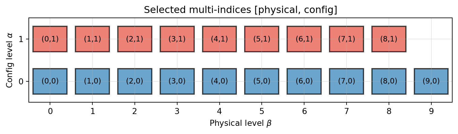
The blue boxes (\(\alpha = 0\)) represent evaluations of the cheap model \(f_0\); the red boxes (\(\alpha = 1\)) represent evaluations of the expensive model \(f_1\). The grid uses more physical levels for the cheap model and fewer for the expensive one.
Animated Refinement
The animation below shows how the adaptive algorithm builds the multi-index set and approximation step by step. Solid boxes are selected (active) subspaces that contribute to the surrogate; dashed boxes are candidates awaiting evaluation and prioritization. When a promoted candidate has no admissible children (due to the downward-closed constraint), the next-best candidate is also promoted in the same step.
Manual Mode: step_samples() / step_values()
For more control, use the manual step pattern. step_samples() returns a dictionary mapping each config index to its required physical samples:
tp_factory2 = TensorProductSubspaceFactory(bkd, phys_factories, growth)
max_1d2 = bkd.asarray([10, 1], dtype=bkd.int64_dtype())
admis2 = CompositeCriteria(
    MaxLevelCriteria(max_level=10, pnorm=1.0, bkd=bkd),
    Max1DLevelsCriteria(max_1d2, bkd),
)
fitter2 = MultiFidelityAdaptiveSparseGridFitter(
    bkd, tp_factory2, admis2, nconfig_vars=1,
)

# Validation samples for true test error
z_val = bkd.array(np.linspace(-1, 1, 500).reshape(1, -1))
exact_val = factory.get_model((1,))(z_val)

error_estimates = []
test_errors = []
for step in range(15):
    config_requests = fitter2.step_samples()
    if config_requests is None:
        break

    # config_requests: {(alpha,): physical_samples}
    values_dict = {}
    for config_idx, phys_samples in config_requests.items():
        model = factory.get_model(config_idx)
        values_dict[config_idx] = model(phys_samples)

    fitter2.step_values(values_dict)
    error_estimates.append(fitter2.current_error())

    # Compute true test error (max abs error on validation grid)
    res2 = fitter2.result()
    approx_val = res2.surrogate(z_val)
    test_err = float(bkd.max(bkd.abs(approx_val - exact_val)))
    test_errors.append(test_err)

    if test_err < 1e-14:
        break
from pyapprox_tutorials.figures._sparse_grids import plot_mf_manual_convergence
fig, ax = plt.subplots(figsize=(8, 4))
steps = range(1, len(error_estimates) + 1)
plot_mf_manual_convergence(ax, steps, error_estimates, test_errors)
plt.tight_layout()
plt.show()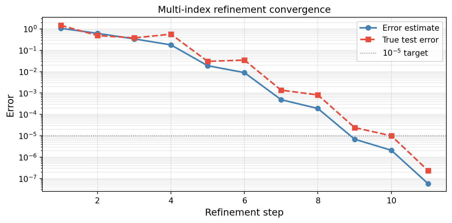
Cost-Aware Refinement
By default, all models are treated as having equal cost (ConstantCostModel). For realistic multi-fidelity problems, the high-fidelity model is far more expensive. ExponentialConfigCostModel assigns cost \(= \text{base}^{\sum \alpha_i}\). All error indicators divide their priority by subspace_cost internally, so swapping in a non-trivial cost_model is enough to make the algorithm prefer refining cheap models first — no separate “cost-weighted wrapper” is needed.
from pyapprox.surrogates.sparsegrids import (
    ExponentialConfigCostModel,
)

cost_model = ExponentialConfigCostModel(base=4.0)
With base 4.0, model \(f_1\) costs 4x more than \(f_0\). The animation below compares the refinement paths of the unit-cost baseline and the fidelity-weighted cost model side by side. Both reach similar final index sets, but the cost-weighted algorithm builds up the cheap model first, deferring the expensive model until its contribution justifies its cost. The cumulative cost shown in each title reveals the practical benefit: the same accuracy is reached at a lower total cost.
The cost-weighted algorithm delays promoting \(\alpha=1\) candidates because their priority is divided by subspace_cost, which for high-fidelity indices includes the 4\(\times\) model-cost factor from ExponentialConfigCostModel. This means it can build up physical resolution with the cheap model before investing in the expensive correction, reaching the same accuracy at lower total cost.
Measured Costs with TimedModelFactory
When model costs are unknown a priori, TimedModelFactory wraps any ModelFactoryProtocol and records wall-clock times for every evaluation. MeasuredCostModel reads these timings to provide data-driven cost estimates that update as the algorithm runs.
from pyapprox.surrogates.sparsegrids import (
    TimedModelFactory,
    MeasuredCostModel,
)

# Wrap our factory with timing instrumentation
timed_factory = TimedModelFactory(factory)
measured_cost = MeasuredCostModel(timed_factory)

# Evaluate some samples to generate timing data
test_samples = bkd.array(np.random.uniform(-1, 1, (1, 100)))
_ = timed_factory.get_model((0,))(test_samples)
_ = timed_factory.get_model((1,))(test_samples)
In a real application where different fidelity levels have genuinely different costs (e.g., coarse vs fine mesh PDE solves), the measured costs would differ significantly, and the cost-weighted indicator would automatically favor the cheaper model.
# Use measured costs with the adaptive fitter
tp_factory_mc = TensorProductSubspaceFactory(bkd, phys_factories, growth)
max_1d_mc = bkd.asarray([10, 1], dtype=bkd.int64_dtype())
admis_mc = CompositeCriteria(
    MaxLevelCriteria(max_level=10, pnorm=1.0, bkd=bkd),
    Max1DLevelsCriteria(max_1d_mc, bkd),
)

# Create a fresh timed factory for the fitter run
timed_factory2 = TimedModelFactory(factory)
measured_cost2 = MeasuredCostModel(timed_factory2)

# The default indicator already cost-weights; just pass the cost model.
fitter_mc = MultiFidelityAdaptiveSparseGridFitter(
    bkd, tp_factory_mc, admis_mc, nconfig_vars=1,
    cost_model=measured_cost2,
)

# The timed_factory is both the model source and the timing recorder
result_mc = fitter_mc.refine_to_tolerance(timed_factory2, tol=1e-6, max_steps=15)
Two-Dimensional Physical + One Config Variable
Here we demonstrate the multi-fidelity approach on a 2D physical problem with two fidelity levels:
\[ f_\alpha(z_1, z_2) = \cos\!\left(\pi z_1 + \epsilon_\alpha\right) \cdot \sin\!\left(\pi z_2 / 2\right), \quad \epsilon_0 = 0.3,\ \epsilon_1 = 0. \]
epsilons_2d = {0: 0.3, 1: 0.0}


def make_2d_model(eps):
    def model(samples):
        z1, z2 = samples[0], samples[1]
        vals = bkd.cos(np.pi * z1 + eps) * bkd.sin(np.pi * z2 / 2)
        return bkd.reshape(vals, (1, -1))
    return model


models_2d = {
    (0,): make_2d_model(epsilons_2d[0]),
    (1,): make_2d_model(epsilons_2d[1]),
}
factory_2d = DictModelFactory(models_2d)

margs_2d = [UniformMarginal(-1.0, 1.0, bkd)] * 2
phys_facs_2d = [GaussLagrangeFactory(m, bkd) for m in margs_2d]
growth_2d = LinearGrowthRule(scale=1, shift=1)
tp_factory_2d = TensorProductSubspaceFactory(bkd, phys_facs_2d, growth_2d)

# Admissibility: 3 index dims = [phys1, phys2, config]
max_1d_2d = bkd.asarray([8, 8, 1], dtype=bkd.int64_dtype())
admis_2d = CompositeCriteria(
    MaxLevelCriteria(max_level=8, pnorm=1.0, bkd=bkd),
    Max1DLevelsCriteria(max_1d_2d, bkd),
)

fitter_2d = MultiFidelityAdaptiveSparseGridFitter(
    bkd, tp_factory_2d, admis_2d, nconfig_vars=1,
)

result_2d = fitter_2d.refine_to_tolerance(factory_2d, tol=1e-8, max_steps=50)
Visualizing the 2D Multi-Index Set
With two physical variables and one configuration variable, each selected subspace index is a triple \([\beta_1, \beta_2, \alpha]\). A 3D scatter plot reveals how the algorithm distributes resolution across the two physical dimensions and the model hierarchy.
from pyapprox_tutorials.figures._sparse_grids import plot_mf_indices_2d

sel_2d = result_2d.indices
sel_2d_np = bkd.to_numpy(sel_2d).astype(int)

fig = plt.figure(figsize=(10, 7))
ax = fig.add_subplot(111, projection="3d")
plot_mf_indices_2d(ax, sel_2d_np)
plt.tight_layout()
plt.show()
The blue markers (\(\alpha = 0\)) span many physical levels using the cheap model, while the red markers (\(\alpha = 1\)) appear at fewer physical levels. The algorithm invests in cheap evaluations first, adding expensive ones only where the discrepancy matters.
Approximation vs True Function
We compare the multi-fidelity surrogate against the true high-fidelity model \(f_1(z_1, z_2)\).
from pyapprox.interface.functions.plot.plot2d_rectangular import (
    Plotter2DRectangularDomain,
)
from pyapprox.interface.functions.fromcallable.function import (
    FunctionFromCallable,
)
from pyapprox_tutorials.figures._sparse_grids import plot_mf_2d_accuracy

plot_limits = [-1.0, 1.0, -1.0, 1.0]

# Build FunctionFromCallable wrappers for plotting
true_fn = FunctionFromCallable(1, 2, make_2d_model(0.0), bkd)

def surrogate_2d_fn(samples):
    return result_2d.surrogate(samples)

surr_fn = FunctionFromCallable(1, 2, surrogate_2d_fn, bkd)

plotter_true = Plotter2DRectangularDomain(true_fn, plot_limits)
plotter_surr = Plotter2DRectangularDomain(surr_fn, plot_limits)

fig, axes = plt.subplots(1, 3, figsize=(16, 4.5))
plot_mf_2d_accuracy(
    axes, fig, plotter_true, plotter_surr, bkd, result_2d,
    true_fn, plot_limits,
)
plt.tight_layout()
plt.show()
Multi-Index with Multiple Config Variables
While this tutorial focuses on a single configuration variable (one-dimensional model hierarchy), the framework naturally extends to multiple configuration variables. As shown in the mesh illustration earlier, a PDE solver might have separate controls for mesh resolution in \(x\) and \(y\):
- Config variable 1: \(x\)-mesh refinement level (\(\alpha_x\))
- Config variable 2: \(y\)-mesh refinement level (\(\alpha_y\))
The nconfig_vars parameter controls this, and Max1DLevelsCriteria specifies the maximum level for each config dimension. The adaptive algorithm then explores the full joint space of physical resolution and model fidelity. With two config variables the index becomes \([\beta_1, \ldots, \beta_d, \alpha_x, \alpha_y]\), and the Smolyak combination builds discrepancy surrogates along each config direction independently.
Summary
- Multi-level collocation approximates \(f_\alpha = f_0 + \sum_{j=1}^{\alpha} (f_j - f_{j-1})\) by interpolating each discrepancy separately. Discrepancies are smoother and cheaper to approximate.
- Multi-index collocation generalizes this to multiple configuration variables using the Smolyak combination over the full (physical + config) index space.
ModelFactoryProtocolrequiresget_model(config_idx). UseDictModelFactoryfor simple cases or implement the protocol directly.MultiFidelityAdaptiveSparseGridFittersupports both auto mode (refine_to_tolerance(model_factory)) and manual mode (step_samples()/step_values()).- Cost-aware refinement via a non-trivial
cost_model(e.g.ExponentialConfigCostModel,MeasuredCostModel) ensures that cheap models are exploited before expensive ones. All error indicators divide priority bysubspace_costinternally, so the cost model alone controls cost-aware behaviour. - Measured costs via
TimedModelFactory+MeasuredCostModelprovide data-driven cost estimates when formula-based costs are unavailable.
Exercises
NoteExercises
Three fidelity levels. Add a third model with \(\epsilon_2 = 0.25\) (intermediate fidelity). Set
max_config_level=2inMax1DLevelsCriteriaand observe how the algorithm distributes evaluations across three models.Cost sensitivity. Change the
baseparameter inExponentialConfigCostModelfrom 4.0 to 2.0 and 10.0. How does this affect the selected multi-index set?Convergence comparison. Compare the multi-fidelity grid against a single-model adaptive grid (using
SingleFidelityAdaptiveSparseGridFitterwith only \(f_1\)). Plot error vs total cost (not just sample count) to see the benefit of multi-fidelity.Measured costs. Modify one of the models to include an artificial
time.sleep()delay and useTimedModelFactory+MeasuredCostModelto verify that the algorithm adapts its priorities based on measured wall times.
Next Steps
This concludes the sparse grid tutorial series. You now have a complete toolkit for:
- Piecewise Polynomial Quadrature — Composite Newton-Cotes rules
- Gauss Quadrature — Optimal nodes from orthogonal polynomials
- Lagrange Interpolation — 1D polynomial interpolation
- Leja Sequences — Nested points for adaptive algorithms
- Piecewise Interpolation — Local basis functions
- Tensor Product Interpolation — Multivariate approximation
- Isotropic Sparse Grids — Breaking the curse of dimensionality
- Adaptive Sparse Grids — Data-driven refinement
- Multifidelity Sparse Grids (this tutorial) — Multi-index collocation
For related topics, see Building a Polynomial Chaos Surrogate for spectral methods and UQ with Polynomial Chaos for moment computation.