---
title: "Bin-Based Sensitivity Analysis"
subtitle: "PyApprox Tutorial Library"
description: "Variance-based sensitivity indices via binning estimation"
tutorial_type: usage
topic: sensitivity_analysis
difficulty: intermediate
estimated_time: 10
render_time: 18
prerequisites:
- sobol_sensitivity_analysis
tags:
- sensitivity-analysis
- sobol-indices
- binning
format:
html:
code-fold: false
code-tools: true
toc: true
execute:
echo: true
warning: false
jupyter: python3
---
::: {.callout-tip collapse="true"}
## Download Notebook
[Download as Jupyter Notebook](notebooks/bin_based_sensitivity.ipynb)
:::
## Learning Objectives
After completing this tutorial, you will be able to:
- Explain the binning estimator for Sobol indices
- Compute main effects and interaction indices from any sample set
- Interpret second-order interaction terms (e.g., $\Sobol{13}$)
- Visualize 2D bin partitions and conditional means
- Compare bin-based vs. sample-based estimators
## Prerequisites
Complete [Sobol Sensitivity Analysis](sobol_sensitivity_analysis.qmd) before this tutorial.
## Why Bin-Based Estimation?
The Saltelli/Jansen estimator for Sobol indices requires a **special sampling design**: two independent sample matrices $\mt{A}$ and $\mt{B}$, plus mixed matrices $\mt{C}_i$. This is efficient when you control sampling, but what if you have an **existing dataset**?
**Bin-based estimation** computes Sobol indices from *any* sample set by:
1. Partitioning each variable's domain into bins using inverse CDF
2. Computing conditional means $\E[Y | X_i \in \text{bin}_k]$ within each bin
3. Computing the variance of these conditional means
This yields the main effect variance $\maineff{i} = \Var[\E[Y|X_i]]$.
## Mathematical Background
### First-Order Index via Binning
Partition $X_i$ into $B$ equal-probability bins using quantiles. For each bin $k$:
$$
\hat{\mu}_k = \frac{1}{n_k} \sum_{j: X_i^{(j)} \in \text{bin}_k} Y^{(j)}
$$
The first-order index estimate is:
$$
\hat{\Sobol{i}} = \frac{\sum_k (n_k / N) (\hat{\mu}_k - \bar{Y})^2}{\hat{\Var}[Y]}
$$
This approximates $\Var[\E[Y|X_i]] / \Var[Y]$.
### Higher-Order Indices
For a second-order index $\Sobol{ij}$, partition *both* $X_i$ and $X_j$ into bins, creating a 2D grid of cells. The raw variance $R_{ij}$ from 2D binning includes contributions from $\Sobol{i}$, $\Sobol{j}$, and the interaction $\Sobol{ij}$:
$$
R_{ij} = \frac{\Var[\E[Y|X_i, X_j]]}{\Var[Y]} = \Sobol{i} + \Sobol{j} + \Sobol{ij}
$$
Therefore:
$$
\Sobol{ij} = R_{ij} - \Sobol{i} - \Sobol{j}
$$
This ANOVA subtraction is handled automatically by `BinBasedSensitivityAnalysis`.
### Key Limitation
**Total effects cannot be computed** via binning. Computing $\SobolT{i}$ would require $(d-1)$-dimensional binning (conditioning on all variables except $X_i$), which is infeasible for $d > 3$ due to the curse of dimensionality.
## Setup
```{python}
import numpy as np
import matplotlib.pyplot as plt
from pyapprox.util.backends.numpy import NumpyBkd
from pyapprox_benchmarks.sensitivity import IshigamiBenchmark
from pyapprox.sensitivity.variance_based import BinBasedSensitivityAnalysis

bkd = NumpyBkd()
np.random.seed(42)

# Load the Ishigami benchmark
benchmark = IshigamiBenchmark(bkd)
func = benchmark.problem().function()
prior = benchmark.problem().prior()

print(f"Ishigami function: f(x) = sin(x1) + 7*sin^2(x2) + 0.1*x3^4*sin(x1)")
print(f"Domain: x_i ~ U[-pi, pi], i = 1,2,3")
```
## First-Order Indices
Let's compute main effects using the bin-based method.
```{python}
# Generate samples from the prior
N = 10000
samples = prior.rvs(N)
values = func(samples)

print(f"Samples shape: {samples.shape}")
print(f"Values shape: {values.shape}")
```
```{python}
# Create bin-based sensitivity analyzer
sa = BinBasedSensitivityAnalysis(prior, bkd)

# Compute sensitivity indices
sa.compute(samples, values)

# Get main effects
main_effects = bkd.to_numpy(sa.main_effects()).flatten()

print("First-order Sobol indices (bin-based estimate):")
for i, s in enumerate(main_effects):
    print(f"  S_{i+1} = {s:.4f}")

print("\nGround truth:")
gt_main = bkd.to_numpy(benchmark.main_effects()).flatten()
for i, s in enumerate(gt_main):
    print(f"  S_{i+1} = {s:.4f}")
```
The bin-based estimates agree reasonably well with the ground truth. The Ishigami function has:
- $X_1$: Moderate main effect through $\sin(X_1)$
- $X_2$: Large main effect through $7\sin^2(X_2)$
- $X_3$: Zero main effect (only appears through interaction $X_3^4 \sin(X_1)$)
## Visualizing 1D Bin Partitions
Let's visualize how the conditional means are computed. First, we prepare the data:
```{python}
# Convert to numpy for visualization
nbins = 10
samples_np = bkd.to_numpy(samples)
values_np = bkd.to_numpy(values).flatten()
global_mean = np.mean(values_np)

def compute_bin_statistics(var_idx, nbins):
    """Compute bin edges and conditional means for one variable."""
    probs = np.linspace(0, 1, nbins + 1)
    bin_edges = np.quantile(samples_np[var_idx], probs)
    bin_indices = np.clip(np.digitize(samples_np[var_idx], bin_edges[:-1]) - 1, 0, nbins - 1)

    bin_means, bin_centers = [], []
    for k in range(nbins):
        mask = bin_indices == k
        if np.sum(mask) > 0:
            bin_means.append(np.mean(values_np[mask]))
            bin_centers.append(np.mean(samples_np[var_idx, mask]))
    return bin_edges, bin_means, bin_centers
```
Now we plot the conditional means for each variable:
```{python}
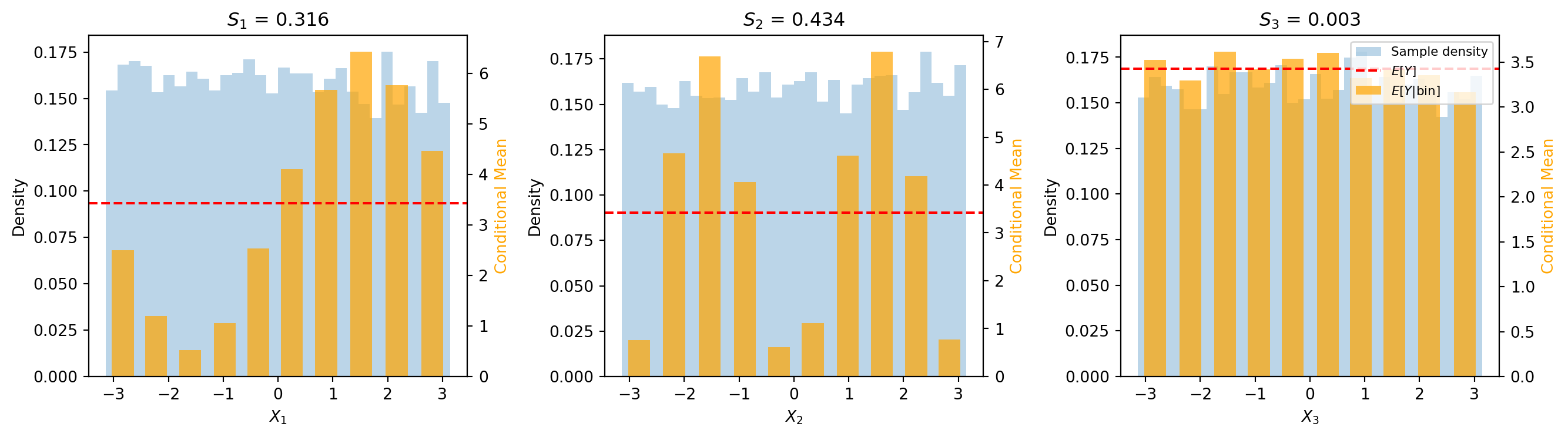
#| fig-cap: "Conditional means per bin for each input variable. Orange bars show the bin-averaged output $\\hat{\\mu}_k = E[Y \\mid X_i \\in \\text{bin}_k]$; the red dashed line marks the global mean $E[Y]$; the blue histogram shows the sample density. Large bar-to-bar variation indicates a high first-order index."
#| label: fig-bin-1d
from pyapprox_tutorials.figures._sensitivity import plot_bin_1d

fig, axes = plt.subplots(1, 3, figsize=(14, 4))
plot_bin_1d(samples_np, values_np, main_effects, nbins, axes)
plt.tight_layout()
plt.show()
```
Note how $X_2$ has the largest variation in conditional means (tallest bars varying from the red line), explaining its high $\Sobol{2}$ value. For $X_3$, the conditional means are nearly constant, giving $\Sobol{3} \approx 0$.
## Second-Order Indices
The Ishigami function has a notable interaction between $X_1$ and $X_3$ through the term $0.1 X_3^4 \sin(X_1)$. Let's compute the second-order index $\Sobol{13}$.
```{python}
# Set up interaction terms of interest (main effects + second-order)
# Interaction matrix: each column is a binary indicator of active variables
# Column 0: [1,0,0] = S_1, Column 1: [0,1,0] = S_2, etc.
interaction_terms = bkd.asarray([
    [1, 0, 0, 1, 1, 0],  # X_1 active in S_1, S_12, S_13
    [0, 1, 0, 1, 0, 1],  # X_2 active in S_2, S_12, S_23
    [0, 0, 1, 0, 1, 1],  # X_3 active in S_3, S_13, S_23
])

sa.set_interaction_terms_of_interest(interaction_terms)
sa.compute(samples, values)

sobol_all = bkd.to_numpy(sa.sobol_indices()).flatten()
print("All Sobol indices:")
print(f"  S_1 = {sobol_all[0]:.4f}")
print(f"  S_2 = {sobol_all[1]:.4f}")
print(f"  S_3 = {sobol_all[2]:.4f}")
print(f"  S_12 = {sobol_all[3]:.4f}")
print(f"  S_13 = {sobol_all[4]:.4f}")
print(f"  S_23 = {sobol_all[5]:.4f}")

print(f"\nGround truth S_13 = {benchmark.sobol_indices().get((0, 2), 'N/A'):.4f}")
print(f"\nSum of all indices = {np.sum(sobol_all):.4f} (should be close to 1)")
```
The $\Sobol{13}$ interaction is substantial (~0.24), capturing the $X_1$-$X_3$ coupling. The other pairwise interactions are near zero.
## Visualizing 2D Bin Partitions
Let's visualize the 2D binning used to compute $\Sobol{13}$. First, we compute the 2D grid of conditional means:
```{python}
# Variables for the X1-X3 interaction
var_i, var_j = 0, 2  # X_1, X_3
nbins_2d = 5

# Get samples for these variables
xi = samples_np[var_i]
xj = samples_np[var_j]

# Compute bin edges using quantiles
edges_i = np.quantile(xi, np.linspace(0, 1, nbins_2d + 1))
edges_j = np.quantile(xj, np.linspace(0, 1, nbins_2d + 1))

# Compute 2D bin indices
bin_i = np.clip(np.digitize(xi, edges_i[:-1]) - 1, 0, nbins_2d - 1)
bin_j = np.clip(np.digitize(xj, edges_j[:-1]) - 1, 0, nbins_2d - 1)

# Compute conditional means for each cell
cell_means = np.zeros((nbins_2d, nbins_2d))
cell_counts = np.zeros((nbins_2d, nbins_2d))

for k in range(N):
    bi, bj = bin_i[k], bin_j[k]
    cell_means[bi, bj] += values_np[k]
    cell_counts[bi, bj] += 1

cell_counts[cell_counts == 0] = 1  # Avoid division by zero
cell_means /= cell_counts

print(f"2D grid: {nbins_2d}x{nbins_2d} = {nbins_2d**2} cells")
print(f"Conditional mean range: [{cell_means.min():.2f}, {cell_means.max():.2f}]")
```
Now we visualize the results:
```{python}
#| fig-cap: "2D binning for the $X_1$--$X_3$ interaction. Left: samples colored by output value with the 5x5 bin grid overlaid. Right: conditional mean $E[Y \\mid X_1, X_3]$ within each cell. The cell-to-cell variation (after subtracting main effects) yields $S_{13}$."
#| label: fig-bin-2d
from pyapprox_tutorials.figures._sensitivity import plot_bin_2d

fig, axes = plt.subplots(1, 2, figsize=(14, 5))
plot_bin_2d(xi, xj, values_np, edges_i, edges_j, cell_means,
            nbins_2d, axes, fig=fig)
plt.tight_layout()
plt.show()
```
The left plot shows samples colored by their $Y$ values with the bin grid overlaid. The right plot shows the conditional mean within each 2D cell. The variation in conditional means across cells (after subtracting main effects) gives the interaction term $\Sobol{13}$.
## Comparison: Bin-Based vs. Sample-Based
Let's compare the bin-based estimates with the Saltelli/Jansen sample-based estimator
**at the same computational budget** (same number of function evaluations).
The sample-based method requires a special sampling design: two independent sample
matrices $\mt{A}$ and $\mt{B}$ (each of size $N_\text{base}$), plus $d$ mixed matrices
$\mt{C}_i$. The total cost is $N_\text{base}(d + 2)$ function evaluations. So for a
budget of $N$ evaluations, the sample-based method can afford $N_\text{base} = \lfloor N / (d + 2) \rfloor$ base samples.
```{python}
from pyapprox.sensitivity import MonteCarloSensitivityAnalysis

gt_main = bkd.to_numpy(benchmark.main_effects()).flatten()
gt_total = bkd.to_numpy(benchmark.total_effects()).flatten()

# Fixed budget: same total number of function evaluations
budgets = [500, 1000, 2000, 5000, 10000]
n_reps = 10

bin_errors = {N: [] for N in budgets}
mc_errors = {N: [] for N in budgets}
mc_total_errors = {N: [] for N in budgets}

for N_budget in budgets:
    for rep in range(n_reps):
        np.random.seed(rep)

        # --- Bin-based: uses all N_budget samples ---
        s = prior.rvs(N_budget)
        v = func(s)
        sa_bin = BinBasedSensitivityAnalysis(prior, bkd)
        sa_bin.compute(s, v)
        bin_main = bkd.to_numpy(sa_bin.main_effects()).flatten()
        bin_errors[N_budget].append(np.max(np.abs(bin_main - gt_main)))

        # --- Sample-based (MC): N_base = N_budget / (d + 2) ---
        d = 3
        N_base = N_budget // (d + 2)
        sa_mc = MonteCarloSensitivityAnalysis(prior, bkd)
        # Only main effects (no pairwise), so nterms = d
        interaction_terms = bkd.asarray(np.eye(d, dtype=float))
        sa_mc.set_interaction_terms_of_interest(interaction_terms)
        mc_samples = sa_mc.generate_samples(N_base)
        mc_values = func(mc_samples)
        sa_mc.compute(mc_values)
        mc_main = bkd.to_numpy(sa_mc.main_effects()).flatten()
        mc_total = bkd.to_numpy(sa_mc.total_effects()).flatten()
        mc_errors[N_budget].append(np.max(np.abs(mc_main - gt_main)))
        mc_total_errors[N_budget].append(np.max(np.abs(mc_total - gt_total)))

# Print summary
print(f"{'Budget':<8}{'Bin max|err|':<18}{'MC max|err| (S)':<18}{'MC max|err| (T)':<18}")
print("-" * 62)
for N_budget in budgets:
    b = np.median(bin_errors[N_budget])
    m = np.median(mc_errors[N_budget])
    t = np.median(mc_total_errors[N_budget])
    print(f"{N_budget:<8}{b:<18.4f}{m:<18.4f}{t:<18.4f}")
```
```{python}
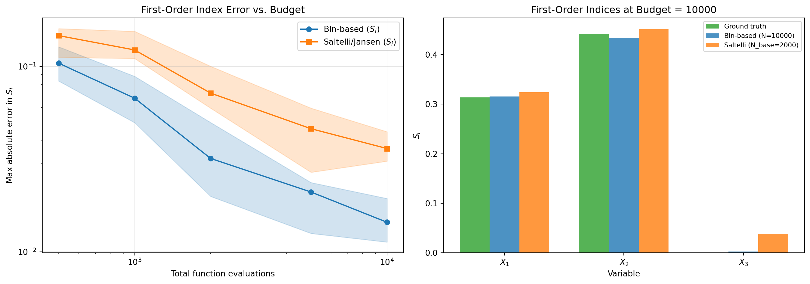
#| fig-cap: "Convergence comparison at equal computational budget. Left: maximum absolute error in first-order Sobol indices vs. number of function evaluations. The bin-based method uses all $N$ samples directly; the sample-based (Saltelli/Jansen) method splits the budget into $N/(d+2)$ base samples. Shaded bands show the 25th--75th percentile range over 10 random seeds. Right: detailed comparison at $N = 10{,}000$ showing per-variable accuracy."
#| label: fig-bin-vs-mc
from pyapprox_tutorials.figures._sensitivity import plot_bin_vs_mc

# Compute detailed comparison at N=10000
N_detail = 10000
np.random.seed(42)

# Bin-based at N_detail
s = prior.rvs(N_detail)
v = func(s)
sa_bin = BinBasedSensitivityAnalysis(prior, bkd)
sa_bin.compute(s, v)
bin_main_detail = bkd.to_numpy(sa_bin.main_effects()).flatten()

# MC at same budget
N_base_detail = N_detail // (3 + 2)
sa_mc = MonteCarloSensitivityAnalysis(prior, bkd)
interaction_terms = bkd.asarray(np.eye(3, dtype=float))
sa_mc.set_interaction_terms_of_interest(interaction_terms)
mc_s = sa_mc.generate_samples(N_base_detail)
mc_v = func(mc_s)
sa_mc.compute(mc_v)
mc_main_detail = bkd.to_numpy(sa_mc.main_effects()).flatten()

fig, axes = plt.subplots(1, 2, figsize=(14, 5))
plot_bin_vs_mc(budgets, bin_errors, mc_errors, gt_main,
               bin_main_detail, mc_main_detail, N_detail,
               N_base_detail, axes)
plt.tight_layout()
plt.show()
```
Both methods converge as the budget increases. The bin-based method uses all $N$ samples
for binning, while the sample-based method must split the budget across its $A$, $B$,
and $C_i$ matrices ($N_\text{base} = N / 5$ for $d = 3$). However, the sample-based
method also provides **total effects**, which binning cannot.
## Bootstrap Uncertainty Estimates
Bin-based estimation has statistical uncertainty. Let's quantify it using bootstrap.
```{python}
# Compute bootstrap statistics
np.random.seed(42)
stats = sa.bootstrap(samples, values, nbootstraps=20, seed=42)

median = bkd.to_numpy(stats['median']).flatten()
q25 = bkd.to_numpy(stats['quantile_25']).flatten()
q75 = bkd.to_numpy(stats['quantile_75']).flatten()

print("Bootstrap statistics for main effects:")
print(f"{'Var':<6}{'Median':<10}{'IQR':<15}{'Std':<10}")
print("-" * 40)
for i in range(3):
    std = bkd.to_numpy(stats['std']).flatten()[i]
    print(f"X_{i+1:<4}{median[i]:<10.4f}[{q25[i]:.4f}, {q75[i]:.4f}]{std:<10.4f}")
```
```{python}
#| fig-cap: "Bootstrap uncertainty of bin-based main effect estimates. Bars show medians over 20 resamples; error bars span the 25th--75th percentile range. Red stars mark the analytical ground truth."
#| label: fig-bootstrap
from pyapprox_tutorials.figures._sensitivity import plot_bootstrap

fig, ax = plt.subplots(figsize=(8, 5))
plot_bootstrap(median, q25, q75, gt_main, ax)
plt.tight_layout()
plt.show()
```
## Trade-offs: Bin-Based vs. Sample-Based
| Aspect | Bin-Based | Saltelli/Jansen |
|--------|-----------|-----------------|
| Sample requirements | Any existing samples | Special A/B/C matrices |
| Cost for $\Sobol{i}$ | $N$ evaluations | $N_\text{base}(d+2)$ evaluations |
| Total effects | Not available | Available |
| Higher-order | Up to ~3rd order | Only first and total |
| Accuracy at equal budget | More samples per estimate | Fewer base samples |
**Use bin-based when:**
- You have existing model evaluations and cannot run new ones
- You need second-order interaction indices
- Total effects are not required
**Use sample-based when:**
- You control the sampling design
- You need total effects
- Maximum efficiency is critical
## Key Takeaways
- **Bin-based estimation** computes Sobol indices from any sample set
- Partitions variables into equal-probability bins using inverse CDF
- **Conditional variance** of bin means approximates $\Var[\E[Y|X_i]]$
- **ANOVA subtraction** extracts pure interaction effects: $\Sobol{ij} = R_{ij} - \Sobol{i} - \Sobol{j}$
- **Total effects infeasible** due to curse of dimensionality in high-order binning
- Bootstrap provides uncertainty quantification
## Exercises
1. **(Easy)** Change the number of bins using `nbins=[15, 4, 3]` (15 bins for 1st order, 4 for 2nd, 3 for 3rd). How do the estimates change?
2. **(Medium)** Perform a convergence study: compute bin-based estimates for $N = 500, 1000, 2000, 5000, 10000$ samples. Plot the error vs. $N$ for each main effect.
3. **(Challenge)** Apply bin-based sensitivity analysis to the 6D Sobol G-function (`sobol_g_6d` benchmark). Compute both main effects and all 15 pairwise interactions. Verify that the sum of indices is close to 1.
## Next Steps
Continue with:
- [PCE-Based Sensitivity](pce_sensitivity.qmd) --- Sobol indices from polynomial chaos surrogates
- [FunctionTrain Sensitivity (Math)](functiontrain_sensitivity_math.qmd) --- Analytical Sobol index derivation from tensor decompositions