import numpy as np
np.random.seed(42)
import matplotlib.pyplot as plt

from pyapprox.util.backends.numpy import NumpyBkd

from pyapprox.surrogates.tensorproduct import TensorProductInterpolant
from pyapprox.surrogates.affine.univariate import (
    LagrangeBasis1D,
    LegendrePolynomial1D,
    GaussQuadratureRule,
)
from pyapprox.surrogates.affine.univariate.globalpoly import (
    ClenshawCurtisQuadratureRule,
)

bkd = NumpyBkd()Tensor Product Interpolation: Multivariate Approximation and Its Limits
PyApprox Tutorial Library
Build multivariate interpolants as tensor products of 1D bases, quantify the curse of dimensionality, and compare Lagrange vs. piecewise convergence in 2D.
TipDownload Notebook
Learning Objectives
After completing this tutorial, you will be able to:
- Construct a multivariate interpolant as a tensor product of 1D Lagrange bases
- Use
TensorProductInterpolantto approximate and evaluate 2D functions - Explain the curse of dimensionality and quantify its impact on point counts
- Compute tensor product quadrature approximations of \(\mathbb{E}[f]\)
- Compare Lagrange vs. piecewise convergence for 2D benchmark functions
Prerequisites
Complete Lagrange Interpolation and Piecewise Polynomial Interpolation before this tutorial.
Setup
The Tensor Product Idea
Given 1D bases \(\{\phi_{1,j_1}\}_{j_1=1}^{M_1}\) and \(\{\phi_{2,j_2}\}_{j_2=1}^{M_2}\) on \([-1,1]\), the tensor product interpolant of a function \(f : [-1,1]^2 \to \mathbb{R}\) is
\[ f_\beta(\mathbf{z}) = \sum_{j_1=1}^{M_1} \sum_{j_2=1}^{M_2} f\!\left(z_1^{(j_1)}, z_2^{(j_2)}\right) \phi_{1,j_1}(z_1)\, \phi_{2,j_2}(z_2). \]
The grid is the Cartesian product of the two 1D node sets: every combination \((z_1^{(j_1)}, z_2^{(j_2)})\) for \(j_1 = 1,\ldots,M_1\) and \(j_2 = 1,\ldots,M_2\). In \(D\) dimensions with \(M\) nodes per dimension, the total number of grid points is \(M^D\) — the source of the curse of dimensionality.
For a \(D\)-dimensional function with \(r\) mixed derivatives the approximation error satisfies
\[ \lVert f - f_\beta \rVert_{\infty} \leq C_{D,r}\, N^{-r/D}, \]
where \(N = M^D\) is the total number of points. The exponent \(1/D\) means that for fixed error tolerance, the required number of points grows exponentially in \(D\).
Constructing a TensorProductInterpolant
TensorProductInterpolant takes a backend, a list of 1D basis objects, and the number of terms per dimension. We demonstrate with \(f(z_1, z_2) = \cos(\pi z_1)\cos(\pi z_2 / 2)\) on \([-1,1]^2\).
def fun_2d(zz):
    """Test function: shape (2, N) → (1, N)"""
    return np.cos(np.pi * zz[0:1]) * np.cos(np.pi * zz[1:2] / 2.0)


# Create 1D Lagrange bases backed by CC quadrature
cc_rule = ClenshawCurtisQuadratureRule(bkd, store=True)
nvars = 2
M = 5  # nodes per dimension (must be valid CC size: 1,3,5,9,17,...)

# Each dimension needs its own basis object
bases_1d = [LagrangeBasis1D(bkd, cc_rule) for _ in range(nvars)]
nterms_1d = [M] * nvars

# Construct the tensor product interpolant
tp = TensorProductInterpolant(bkd, bases_1d, nterms_1d)

# Get the grid points and evaluate the function
grid = tp.get_samples()   # (2, M^2)
values = bkd.array(fun_2d(bkd.to_numpy(grid)))   # (1, M^2)
tp.set_values(values)

# Evaluate on a fine mesh
nfine = 51
z1f = np.linspace(-1, 1, nfine)
z2f = np.linspace(-1, 1, nfine)
z1g, z2g = np.meshgrid(z1f, z2f)
eval_pts = bkd.array(np.vstack([z1g.ravel(), z2g.ravel()]))
tp_vals = bkd.to_numpy(tp(eval_pts))              # (1, nfine^2)
true_vals = fun_2d(np.vstack([z1g.ravel(), z2g.ravel()]))
from pyapprox_tutorials.figures._interpolation import plot_tp_2d
grid_np = bkd.to_numpy(grid)
Z_true = true_vals.reshape(nfine, nfine)
Z_interp = tp_vals.reshape(nfine, nfine)
fig, axs = plt.subplots(1, 3, figsize=(15, 5))
plot_tp_2d(Z_true, Z_interp, grid_np, M, nfine, axs)
plt.tight_layout()
plt.show()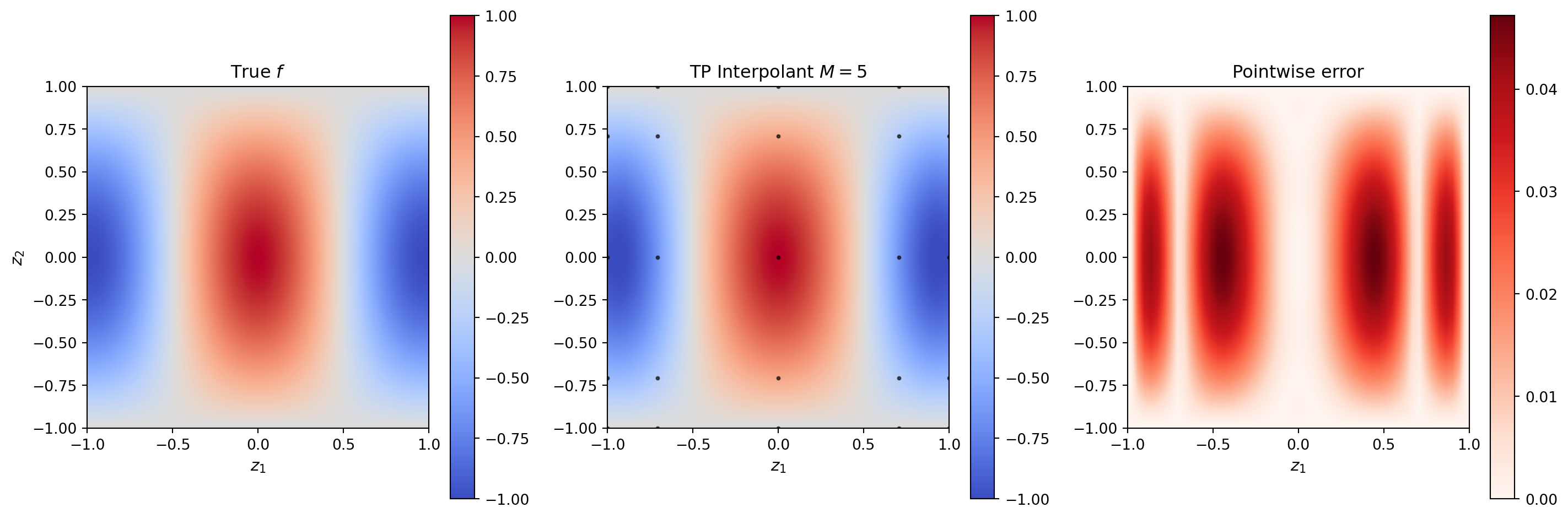
The Curse of Dimensionality
The fundamental problem with tensor products is captured in the point-count table below. For \(M\) nodes per dimension and \(D\) dimensions, the grid has \(M^D\) points. Even at \(M = 3\) nodes per dimension, the count explodes past \(10^4\) for \(D = 9\).
from pyapprox_tutorials.figures._interpolation import plot_curse_of_dimensionality

dims  = [2, 3, 4, 6, 10]
levels = np.arange(0, 6)

fig, ax = plt.subplots(figsize=(9, 5))
plot_curse_of_dimensionality(levels, dims, ax)
plt.tight_layout()
plt.show()
Tensor Product Quadrature
Integrating the tensor product interpolant analytically yields a tensor product quadrature rule. The weights are the products of the 1D quadrature weights:
\[ \mathbb{E}[f(\mathbf{z})] \approx \sum_{j_1=1}^{M} \cdots \sum_{j_D=1}^{M} f\!\left(z_1^{(j_1)}, \ldots, z_D^{(j_D)}\right) \prod_{i=1}^{D} w_i^{(j_i)}. \]
This is equivalent to applying the 1D quadrature rule in each dimension independently.
# Build TP interpolant on CC nodes and compute E[f] via quadrature
M_q = 9
bases_q = [LagrangeBasis1D(bkd, cc_rule) for _ in range(2)]
tp_q = TensorProductInterpolant(bkd, bases_q, [M_q, M_q])

grid_q = tp_q.get_samples()
vals_q = bkd.array(fun_2d(bkd.to_numpy(grid_q)))
tp_q.set_values(vals_q)

# Get 1D CC weights
_, w1d = cc_rule(M_q)                         # (M_q, 1)
w1d_np = bkd.to_numpy(w1d).ravel()            # prob measure, sum to 1

# TP weights: outer product of 1D weights
ww = np.outer(w1d_np, w1d_np).ravel()         # (M_q^2,)
vals_q_np = bkd.to_numpy(vals_q).ravel()

integral_tp = ww @ vals_q_np
# True E[f] = E[cos(pi*z1)] * E[cos(pi*z2/2)] = 0 * (2/pi) = 0
true_int = 0.0
Convergence: Lagrange vs. Piecewise in 2D
We compare the convergence of tensor product interpolants based on Clenshaw-Curtis (Lagrange) and piecewise-linear bases for a smooth and a non-smooth 2D function.
from pyapprox.surrogates.affine.univariate import PiecewiseLinear
from pyapprox_tutorials.figures._interpolation import plot_2d_convergence

def fun_smooth_2d(zz):
    return np.exp(-0.5 * (zz[0:1]**2 + zz[1:2]**2))

def fun_nonsmooth_2d(zz):
    return np.maximum(0.0, zz[0:1] + zz[1:2])


nfine_ref = 100
z1r = np.linspace(-1, 1, nfine_ref)
z2r = np.linspace(-1, 1, nfine_ref)
z1rg, z2rg = np.meshgrid(z1r, z2r)
eval_ref = bkd.array(np.vstack([z1rg.ravel(), z2rg.ravel()]))
eval_ref_np = bkd.to_numpy(eval_ref)

funcs = [
    (fun_smooth_2d,    r"$e^{-(z_1^2+z_2^2)/2}$ — analytic"),
    (fun_nonsmooth_2d, r"$\max(0, z_1+z_2)$ — $C^0$ kink"),
]

# CC Lagrange: use valid CC sizes
Ms_cc = [3, 5, 9, 17]
# Piecewise linear: any M works
Ms_pw = [3, 5, 9, 17, 33]

err_cc_smooth, err_cc_nonsmooth = [], []
err_pw_smooth, err_pw_nonsmooth = [], []
func_labels = []

for func, label in funcs:
    true_ref2d = func(eval_ref_np)
    err_cc, err_pw = [], []

    # CC Lagrange TP
    for M2 in Ms_cc:
        bases_cc = [LagrangeBasis1D(bkd, cc_rule) for _ in range(2)]
        tp_cc = TensorProductInterpolant(bkd, bases_cc, [M2, M2])
        grid_cc = tp_cc.get_samples()
        vals_cc = bkd.array(func(bkd.to_numpy(grid_cc)))
        tp_cc.set_values(vals_cc)
        interp_cc = bkd.to_numpy(tp_cc(eval_ref))
        err_cc.append(np.max(np.abs(interp_cc - true_ref2d)))

    # Piecewise linear TP (manual — TPI requires InterpolationBasis1DProtocol)
    for M2 in Ms_pw:
        nodes_pw = np.linspace(-1, 1, M2)
        z1pw, z2pw = np.meshgrid(nodes_pw, nodes_pw)
        grid_pw_np = np.vstack([z1pw.ravel(), z2pw.ravel()])
        gv_pw = func(grid_pw_np).reshape(M2, M2)

        nodes_bkd = bkd.array(nodes_pw)
        pw_basis = PiecewiseLinear(nodes_bkd, bkd)
        phi1 = bkd.to_numpy(pw_basis(bkd.array(eval_ref_np[0])))  # (nref, M2)
        phi2 = bkd.to_numpy(pw_basis(bkd.array(eval_ref_np[1])))  # (nref, M2)
        interp_pw = np.einsum("ni,nj,ij->n", phi1, phi2, gv_pw)
        err_pw.append(np.max(np.abs(interp_pw - true_ref2d.ravel())))

    if "analytic" in label:
        err_cc_smooth, err_pw_smooth = err_cc, err_pw
    else:
        err_cc_nonsmooth, err_pw_nonsmooth = err_cc, err_pw
    func_labels.append(label)

fig, axs = plt.subplots(1, 2, figsize=(13, 5))
plot_2d_convergence(Ms_cc, err_cc_smooth, err_cc_nonsmooth,
                    Ms_pw, err_pw_smooth, err_pw_nonsmooth,
                    func_labels, axs)
plt.suptitle("2D tensor product convergence", fontsize=13, y=1.01)
plt.tight_layout()
plt.show()
For the analytic function CC converges exponentially until machine precision; for the non-smooth function both methods converge algebraically, with piecewise linear slightly worse in maximum norm but without the spurious oscillations that a high-\(M\) Lagrange basis would produce.
Key Takeaways
- The tensor product interpolant evaluates \(f\) at the Cartesian product of 1D node sets and combines 1D basis functions multiplicatively.
- Point counts scale as \(M^D\): even moderate \(D\) and \(M\) produce grids with millions of evaluations, making tensor products infeasible beyond \(D \approx 4\).
- Tensor product quadrature weights are products of 1D weights; expectations can be computed as a dot product over the grid.
- For smooth functions, CC Lagrange tensor products achieve exponential convergence; for non-smooth functions, piecewise bases are more robust.
- The curse of dimensionality motivates sparse grids (Tutorial 6), which achieve much better point efficiency by omitting high-order cross-terms.
Exercises
NoteExercises
Grid counts. For error tolerance \(\epsilon = 10^{-6}\) and the analytic function \(e^{-(z_1^2+z_2^2)/2}\), estimate the number of TP grid points needed in \(D = 2, 3, 4\). At what \(D\) does the count exceed \(10^6\)?
Anisotropic TP. Use \(M_1 = 17\) nodes in \(z_1\) and \(M_2 = 5\) nodes in \(z_2\) for \(f(z_1, z_2) = \cos(5\pi z_1) + 0.1 z_2\). Compare the error against an isotropic \(M_1 = M_2 = 9\) grid with the same total point count.
Quadrature dimension scaling. Compute \(\mathbb{E}[e^{-(z_1^2+\ldots+z_D^2)/2}]\) for \(D = 2, 3, 4\) using TP Gauss quadrature with \(M = 7\) per dimension. Compare against the known analytic value.
Piecewise tensor product. Use a piecewise quadratic tensor product to approximate \(\max(0, z_1 + z_2)\) and compare the convergence rate with piecewise linear.
Next Steps
- Isotropic Sparse Grids — The Smolyak combination technique recovers near-optimal convergence with exponentially fewer points
- Adaptive Sparse Grids — Data-driven refinement for anisotropic functions