---
title: "General ACV: Analysis"
subtitle: "PyApprox Tutorial Library"
description: "From the two-model ACV derivation through the general optimal weight matrix, the Schur complement variance reduction, and the allocation-matrix framework that parametrises all ACV estimators."
tutorial_type: analysis
topic: multi_fidelity
difficulty: intermediate
estimated_time: 25
render_time: 196
prerequisites:
- acv_many_models_concept
- mfmc_analysis
tags:
- multi-fidelity
- acv
- optimal-weights
- estimator-theory
- allocation-matrix
format:
html:
code-fold: false
code-tools: true
toc: true
execute:
echo: true
warning: false
jupyter: python3
---
::: {.callout-tip collapse="true"}
## Download Notebook
[Download as Jupyter Notebook](notebooks/acv_many_models_analysis.ipynb)
:::
## Learning Objectives
After completing this tutorial, you will be able to:
- Derive the two-model ACV optimal weight $\eta^*$, variance reduction factor, and
optimal sample ratio $r^*$ for a fixed budget
- Write the general ACV estimator for a vector-valued statistic with $M$ LF models
- Derive the optimal weight matrix $\mathbf{H}^* = -\Sigma_{\Delta\Delta}^{-1}\Sigma_{\Delta Q_0}$
and the resulting minimum covariance
- Identify $\Sigma_{\Delta\Delta}$ and $\Sigma_{\Delta Q_0}$ as the two quantities that
determine every ACV estimator's variance
- State how the allocation matrix parameterises the sample-set structure and reduces
the optimisation to a tractable form
- Verify the theoretical variance numerically for MLMC, MFMC, and ACVMF
## Prerequisites
Complete [General ACV Concept](acv_many_models_concept.qmd) and
[MFMC Analysis](mfmc_analysis.qmd) before this tutorial.
## Warm-Up: The Two-Model Case {#sec-two-model}
Before tackling the general multi-model framework, we derive the key results for the
simplest ACV estimator: one HF model $f_\alpha$ and one LF model $f_\kappa$.
### Setup and notation
Let $C_\alpha, C_\kappa$ be per-sample costs and define population moments
$$
\sigma^2_\alpha = \mathbb{V}[f_\alpha], \quad
\sigma^2_\kappa = \mathbb{V}[f_\kappa], \quad
C_{\alpha\kappa} = \mathrm{Cov}(f_\alpha, f_\kappa), \quad
\rho_{\alpha\kappa} = \frac{C_{\alpha\kappa}}{\sigma_\alpha \sigma_\kappa}.
$$
Draw $N$ shared samples $\mathcal{Z}_N$ and $rN$ LF-only samples
$\mathcal{Z}_{rN} \supset \mathcal{Z}_N$ ($r > 1$). The ACV estimator is
$$
\hat{\mu}_\alpha^{\text{ACV}} = \hat{\mu}_\alpha + \eta\left(\hat{\mu}_\kappa^N - \hat{\mu}_\kappa^{rN}\right).
$$ {#eq-acv-two}
### Variance of the correction term
Split $\hat{\mu}_\kappa^{rN}$ into the shared and exclusive parts. The two parts use
**disjoint** sample sets, so they are independent:
$$
\mathbb{V}\!\left[\hat{\mu}_\kappa^N - \hat{\mu}_\kappa^{rN}\right]
= \frac{(r-1)^2}{r^2}\cdot\frac{\sigma^2_\kappa}{N}
+ \frac{1}{r^2}\cdot\frac{\sigma^2_\kappa}{N}
= \frac{r-1}{r}\cdot\frac{\sigma^2_\kappa}{N}.
$$ {#eq-correction-var}
### Optimal weight and variance reduction
The ACV estimator variance is quadratic in $\eta$. Setting the derivative to zero:
$$
\eta^* = -\frac{C_{\alpha\kappa}}{\sigma^2_\kappa}.
$$ {#eq-eta-star-two}
This is **identical** to the CVMC optimal weight — the extra LF samples do not change the
optimal correction direction, only the precision of the correction. Substituting $\eta^*$:
$$
\boxed{
\mathbb{V}\!\left[\hat{\mu}_\alpha^{\text{ACV}}\right]
= \frac{\sigma^2_\alpha}{N}\left(1 - \frac{r-1}{r}\,\rho^2_{\alpha\kappa}\right).
}
$$ {#eq-acv-var-two}
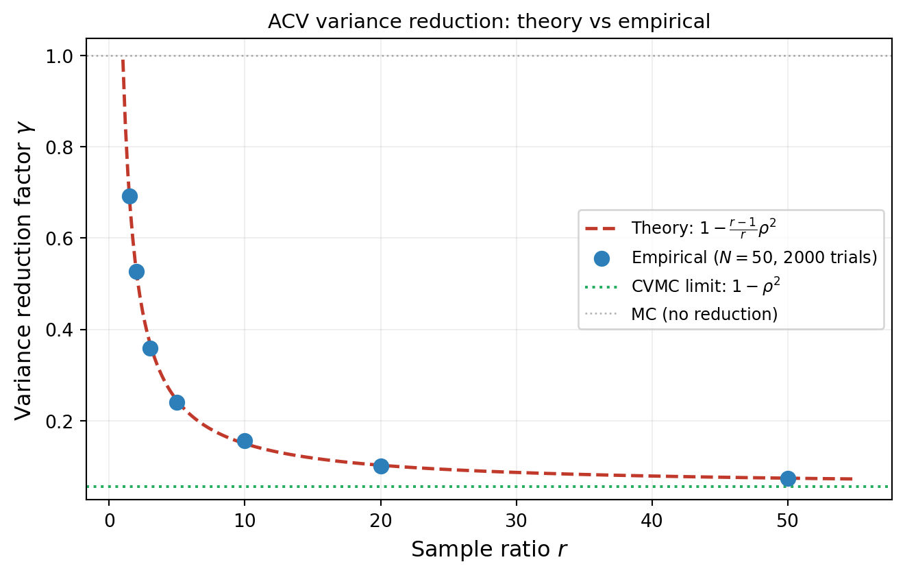
The variance reduction factor is $\gamma = 1 - \frac{r-1}{r}\rho^2_{\alpha\kappa}$, which
interpolates between no reduction ($r \to 1$) and full CVMC reduction ($r \to \infty$).
### Optimal sample allocation for a fixed budget
For total budget $P$ with cost constraint $N C_\alpha + r N C_\kappa = P$, the
estimator variance as a function of $r$ alone is
$$
\mathbb{V}\!\left[\hat{\mu}_\alpha^{\text{ACV}}\right]
= \frac{\sigma^2_\alpha (C_\alpha + r C_\kappa)}{P}
\left(1 - \frac{r-1}{r}\rho^2_{\alpha\kappa}\right).
$$
Minimising over $r > 1$:
$$
r^* = \sqrt{\frac{C_\alpha}{C_\kappa}\cdot\frac{\rho^2_{\alpha\kappa}}{1 - \rho^2_{\alpha\kappa}}}.
$$ {#eq-r-star}
When $\rho_{\alpha\kappa}$ is large and $C_\kappa$ is small, the optimal $r^*$ is large —
many cheap LF samples are worth buying to tighten the correction.
### Numerical verification
```{python}
#| fig-cap: "Empirical ACV variance reduction (dots) versus the theoretical prediction $1 - \\frac{r-1}{r}\\rho^2$ (dashed line) across a range of sample ratios $r$. Each point uses $N = 50$ HF samples and 2000 independent trials."
#| label: fig-acv-verification
import numpy as np
import matplotlib.pyplot as plt
from pyapprox.util.backends.numpy import NumpyBkd
from pyapprox_benchmarks.statest import (
    TunableEnsembleBenchmark,
)
from pyapprox.statest.statistics import MultiOutputMean
from pyapprox.statest.acv import MFMCEstimator
from pyapprox.statest.acv.allocation import ACVAllocationResult
from pyapprox.statest.acv.base import FittedACVEstimator

bkd = NumpyBkd()
benchmark = TunableEnsembleBenchmark(bkd, theta1=np.pi / 2 * 0.95)
hf_model  = benchmark.problem().models()[0]
lf_model  = benchmark.problem().models()[1]
variable  = benchmark.problem().prior()
nqoi      = hf_model.nqoi()

cov_exact     = benchmark.ensemble_covariance()[:2, :2]
cov_mat       = bkd.to_numpy(cov_exact)
sigma2_alpha  = cov_mat[0, 0]
sigma2_kappa  = cov_mat[1, 1]
C_alphakappa  = cov_mat[0, 1]
rho           = C_alphakappa / np.sqrt(sigma2_alpha * sigma2_kappa)

stat = MultiOutputMean(nqoi, bkd)
stat.set_pilot_quantities(cov_exact)

N        = 50
n_trials = 2000
r_values = [1.5, 2, 3, 5, 10, 20, 50]
mc_var   = sigma2_alpha / N

cost_hf_unit = 1.0
cost_lf_unit = 0.001

empirical_reductions = []

for r in r_values:
    est = MFMCEstimator(stat, costs=[cost_hf_unit, cost_lf_unit])
    target_cost = N * cost_hf_unit + r * N * cost_lf_unit
    partition_ratios = bkd.asarray([float(r - 1)])
    npart = est._npartition_samples_from_partition_ratios(
        target_cost, partition_ratios
    )
    npart_int = bkd.asarray(
        [int(round(float(npart[k]))) for k in range(len(npart))],
        dtype=int,
    )
    nsamp = bkd.asarray(
        [int(round(float(v))) for v in est._compute_nsamples_per_model(npart)],
        dtype=int,
    )
    actual_cost = float((nsamp * bkd.asarray([cost_hf_unit, cost_lf_unit])).sum())
    alloc = ACVAllocationResult(
        partition_ratios=partition_ratios,
        continuous_npartition_samples=npart,
        objective_value=bkd.asarray([0.0]),
        npartition_samples=npart_int,
        nsamples_per_model=nsamp,
        target_cost=target_cost,
        actual_cost=actual_cost,
        success=True,
    )
    fitted = FittedACVEstimator(est, alloc)

    acv_ests = np.empty(n_trials)
    for i in range(n_trials):
        np.random.seed(i)
        s_hf, s_lf = fitted.generate_samples_per_model(variable.rvs)
        acv_ests[i] = bkd.to_numpy(
            fitted([hf_model(s_hf), lf_model(s_lf)])
        )[0]
    empirical_reductions.append(np.var(acv_ests) / mc_var)

r_fine = np.linspace(1.01, 55, 300)
theory_line = 1 - (r_fine - 1) / r_fine * rho**2

from pyapprox_tutorials.figures._cv_acv import plot_acv_two_model_verification

fig, ax = plt.subplots(figsize=(7, 4.5))
plot_acv_two_model_verification(r_values, empirical_reductions, rho,
                                N, n_trials, ax)
plt.tight_layout()
plt.show()
```
## The General ACV Estimator
We now generalise from the two-model case to $M$ low-fidelity models. Let $f_0, \ldots, f_M$
be models and let $\mathbf{Q}_0 \in \mathbb{R}^S$ be a vector-valued statistic of the
high-fidelity model. Each low-fidelity model $f_\alpha$ ($\alpha = 1, \ldots, M$)
contributes a **correction vector**
$$
\boldsymbol{\Delta}_\alpha = \mathbf{Q}_\alpha(\mathcal{Z}_\alpha^*) - \mathbf{Q}_\alpha(\mathcal{Z}_\alpha),
$$
where $\mathcal{Z}_\alpha^*$ and $\mathcal{Z}_\alpha$ are two sample sets that may or
may not overlap. Each $\boldsymbol{\Delta}_\alpha$ is unbiased for zero regardless of
the sample-set structure.
Stack the corrections into a single vector
$\boldsymbol{\Delta} = [\boldsymbol{\Delta}_1^\top, \ldots, \boldsymbol{\Delta}_M^\top]^\top \in \mathbb{R}^{SM}$.
The **general ACV estimator** is
$$
\hat{\mathbf{Q}}_0^{\text{ACV}} = \mathbf{Q}_0(\mathcal{Z}_0) + \mathbf{H}\,\boldsymbol{\Delta},
$$ {#eq-acv-general}
where $\mathbf{H} \in \mathbb{R}^{S \times SM}$ is the weight matrix. Because each
$\boldsymbol{\Delta}_\alpha$ has zero mean, the estimator is unbiased for any $\mathbf{H}$.
::: {.callout-note}
## Special cases
When $S = 1$ and $M = 1$, @eq-acv-general reduces to @eq-acv-two from the warm-up.
MLMC, MFMC, and ACVMF are all instances of @eq-acv-general with different choices of
sample-set structure (encoded by the allocation matrix) and different $\mathbf{H}$.
:::
## Covariance of the ACV Estimator
Define the covariance blocks
$$
\Sigma_{\Delta\Delta} = \mathbb{C}\mathrm{ov}(\boldsymbol{\Delta}, \boldsymbol{\Delta}) \in \mathbb{R}^{SM \times SM},
\qquad
\Sigma_{\Delta Q_0} = \mathbb{C}\mathrm{ov}(\boldsymbol{\Delta}, \mathbf{Q}_0) \in \mathbb{R}^{SM \times S}.
$$
Using the variance-of-sums formula:
$$
\mathbb{C}\mathrm{ov}(\hat{\mathbf{Q}}_0^{\text{ACV}}) =
\Sigma_{Q_0 Q_0}
+ \mathbf{H}\,\Sigma_{\Delta\Delta}\,\mathbf{H}^\top
+ \mathbf{H}\,\Sigma_{\Delta Q_0}
+ \Sigma_{Q_0 \Delta}\,\mathbf{H}^\top,
$$ {#eq-acv-cov}
where $\Sigma_{Q_0 Q_0} = \mathbb{C}\mathrm{ov}(\mathbf{Q}_0(\mathcal{Z}_0))$ and
$\Sigma_{Q_0\Delta} = \Sigma_{\Delta Q_0}^\top$.
How to compute $\Sigma_{\Delta\Delta}$ and $\Sigma_{\Delta Q_0}$ from model covariances
and the sample-set intersection sizes is derived in @sec-covariance-formulas.
## Optimal Weight Matrix
@eq-acv-cov is a quadratic function of $\mathbf{H}$. Differentiating and setting to zero:
$$
\mathbf{H}^* = -\Sigma_{\Delta Q_0}^\top \Sigma_{\Delta\Delta}^{-1}.
$$ {#eq-eta-star}
This is the direct multi-model generalisation of the scalar two-model optimal weight
@eq-eta-star-two.
Substituting $\mathbf{H}^*$ back into @eq-acv-cov gives the **minimum ACV covariance**:
$$
\boxed{
\mathbb{C}\mathrm{ov}(\hat{\mathbf{Q}}_0^{\text{ACV}})
= \Sigma_{Q_0 Q_0}
- \Sigma_{Q_0\Delta}\,\Sigma_{\Delta\Delta}^{-1}\,\Sigma_{\Delta Q_0}.
}
$$ {#eq-acv-min-cov}
The variance reduction is the **Schur complement**
$\Sigma_{Q_0\Delta}\,\Sigma_{\Delta\Delta}^{-1}\,\Sigma_{\Delta Q_0}$, which is always
positive semidefinite. ACV can never *increase* variance with optimal weights.
::: {.callout-important}
## What determines variance reduction
@eq-acv-min-cov shows that variance reduction depends on two things only:
$\Sigma_{Q_0\Delta}$ (how well each correction correlates with $\mathbf{Q}_0$) and
$\Sigma_{\Delta\Delta}$ (how noisy each correction is, and how they covary with each
other). The allocation matrix controls both through the sample-set intersection sizes.
:::
## From Theory to Practice: The Allocation Matrix {#sec-allocation-matrix}
For a general sample allocation, computing $\Sigma_{\Delta\Delta}$ and
$\Sigma_{\Delta Q_0}$ requires knowing all pairwise set intersection sizes. Optimising
over all possible values simultaneously is intractable.
All practical ACV methods restrict the search space by requiring sample sets to be unions
of $M+1$ **independent partitions** $\mathcal{P}_0, \ldots, \mathcal{P}_M$, each of size
$p_m$. The **allocation matrix** $\mathbf{A} \in \{0,1\}^{(M+1) \times 2(M+1)}$ encodes
which partitions are included in which sets:
$$
A_{m, 2\alpha-1} = 1 \iff \mathcal{P}_m \subseteq \mathcal{Z}_\alpha^*, \qquad
A_{m, 2\alpha} = 1 \iff \mathcal{P}_m \subseteq \mathcal{Z}_\alpha.
$$
The first column ($\mathcal{Z}_0^*$) is always all-zeros. Given $\mathbf{A}$, any
pairwise intersection size is the weighted inner product of two binary column vectors:
$$
|\mathcal{Z}_j \cap \mathcal{Z}_k| = \mathbf{a}_j^\top \mathrm{diag}(\mathbf{p})\, \mathbf{a}_k.
$$ {#eq-intersection}
This makes $\Sigma_{\Delta\Delta}(\mathbf{p})$ and $\Sigma_{\Delta Q_0}(\mathbf{p})$
tractable functions of the partition sizes, and the optimal allocation becomes the problem
$$
\min_{\mathbf{p}}\;
\det\!\left[\Sigma_{Q_0 Q_0}
- \Sigma_{Q_0\Delta}(\mathbf{p})\,\Sigma_{\Delta\Delta}(\mathbf{p})^{-1}\,\Sigma_{\Delta Q_0}(\mathbf{p})
\right]
\quad \text{subject to} \quad
\sum_{m=0}^M p_m C_{m}(\mathbf{A}) \leq P,
$$ {#eq-alloc-opt}
solved numerically by `ACVAllocator` in PyApprox.
### Allocation matrix examples
The **two-model ACV** from @sec-two-model has two partitions ($\mathcal{P}_0$: shared,
$\mathcal{P}_1$: LF-exclusive):
$$
\mathbf{A}_{\text{ACV}} =
\begin{pmatrix}
0 & 1 & 1 & 1 \\
0 & 0 & 0 & 1
\end{pmatrix}.
$$
For three models, the **MFMC** and **ACVMF** allocation matrices are:
$$
\mathbf{A}_{\text{MFMC}} =
\begin{pmatrix}
0 & 1 & 1 & 1 & 1 & 1 & 1 & 1 \\
0 & 0 & 0 & 1 & 1 & 1 & 1 & 1 \\
0 & 0 & 0 & 0 & 0 & 1 & 1 & 1 \\
0 & 0 & 0 & 0 & 0 & 0 & 0 & 1
\end{pmatrix},
\qquad
\mathbf{A}_{\text{ACVMF}} =
\begin{pmatrix}
0 & 1 & 1 & 1 & 1 & 1 & 1 & 1 \\
0 & 0 & 0 & 1 & 0 & 1 & 0 & 1 \\
0 & 0 & 0 & 0 & 0 & 1 & 0 & 1 \\
0 & 0 & 0 & 0 & 0 & 0 & 0 & 1
\end{pmatrix}.
$$
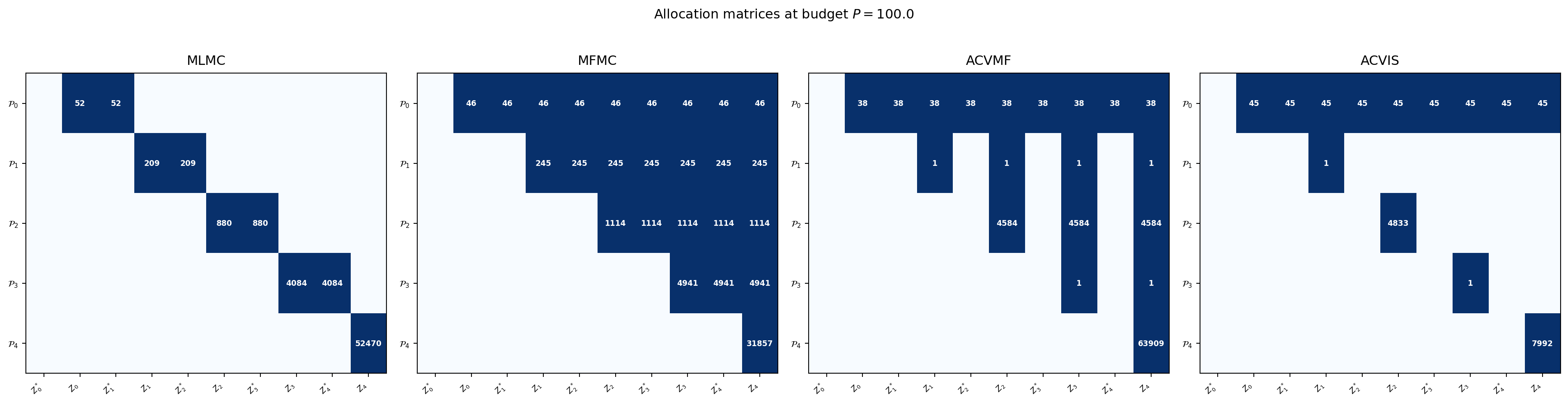
In ACVMF, partition $\mathcal{P}_0$ appears in the $\mathcal{Z}_\alpha^*$ column of
**every** LF model — making all corrections directly correlated with
$\hat{\mu}_0(\mathcal{Z}_0)$ and enabling the full Schur complement reduction.
### Visualising allocation matrices
```{python}
#| fig-cap: "Allocation matrices for MLMC, MFMC, ACVMF, and ACVIS at budget $P = 100$. Each row is a partition $\\mathcal{P}_m$; each column pair is $(\\mathcal{Z}_\\alpha^*, \\mathcal{Z}_\\alpha)$. Numbers show optimised partition sizes."
#| label: fig-allocation-matrices
import numpy as np
np.random.seed(42)
import matplotlib.pyplot as plt
from pyapprox.util.backends.numpy import NumpyBkd
from pyapprox_benchmarks.statest import (
    PolynomialEnsembleBenchmark,
)
from pyapprox.statest.statistics import MultiOutputMean
from pyapprox.statest import (
    MCEstimator, MLMCEstimator, MFMCEstimator, GMFEstimator, GISEstimator,
)
from pyapprox.statest.acv import (
    ACVAllocator, default_allocator_factory,
)
from pyapprox.statest.acv.base import FittedACVEstimator
from pyapprox.statest.allocation import MCAllocator
from pyapprox.optimization.minimize.scipy.slsqp import (
    ScipySLSQPOptimizer,
)

bkd       = NumpyBkd()
benchmark = PolynomialEnsembleBenchmark(bkd, nmodels=5)
models    = benchmark.problem().models()
costs     = benchmark.problem().costs()
nqoi      = models[0].nqoi()
n_models  = len(models)
M         = n_models - 1

stat = MultiOutputMean(nqoi, bkd)
stat.set_pilot_quantities(bkd.asarray(bkd.to_numpy(benchmark.ensemble_covariance())))

target_cost = 100.0
ri_zeros = bkd.zeros(M, dtype=int)

optimizer = ScipySLSQPOptimizer(maxiter=200)

templates = {
    "MLMC":  MLMCEstimator(stat, costs),
    "MFMC":  MFMCEstimator(stat, costs),
    "ACVMF": GMFEstimator(stat, costs, recursion_index=ri_zeros),
    "ACVIS": GISEstimator(stat, costs, recursion_index=ri_zeros),
}
estimators = {}
for name, est in templates.items():
    if name in ("MLMC", "MFMC"):
        allocator = default_allocator_factory(est)
    else:
        allocator = ACVAllocator(est, optimizer=optimizer)
    estimators[name] = FittedACVEstimator(est, allocator.allocate(target_cost))

from pyapprox_tutorials.figures._cv_acv import plot_allocation_matrices

fig, axes = plt.subplots(1, 4, figsize=(20, 5))
plot_allocation_matrices(estimators, bkd, axes)
plt.suptitle(f"Allocation matrices at budget $P = {target_cost}$", fontsize=12, y=1.02)
plt.tight_layout()
plt.show()
```
## Numerical Verification
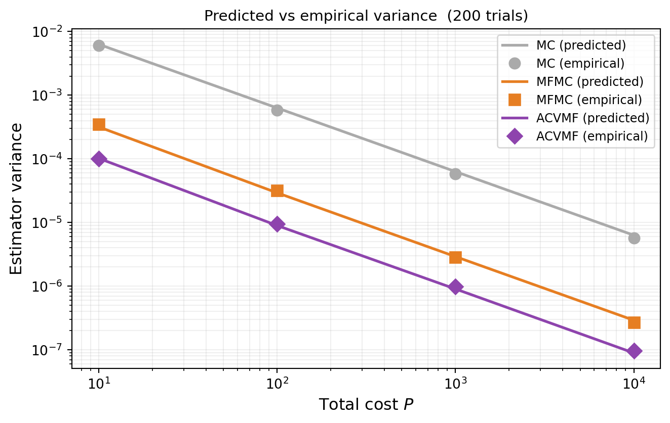
We verify @eq-acv-min-cov by comparing predicted variance from `covariance()`
against empirical variance from independent trials.
```{python}
#| fig-cap: "MC, MFMC, and ACVMF variance vs total cost: predictions (lines) compared to empirical variance from 200 independent trials (markers)."
#| label: fig-variance-verify
variable  = benchmark.problem().prior()

opt_verify = ScipySLSQPOptimizer(maxiter=200)

target_costs_sweep = [10, 100, 1000, 10000]
n_trials = 200

mc_vars_pred, mfmc_vars_pred, acvmf_vars_pred = [], [], []
mc_vars_emp, mfmc_vars_emp, acvmf_vars_emp = [], [], []

def rvs_int(n):
    return variable.rvs(int(n))

for P_t in target_costs_sweep:
    # --- Predicted variance ---
    mc_e = MCEstimator(stat, costs)
    mc_fitted = MCAllocator(mc_e).allocate(float(P_t))
    mc_vars_pred.append(float(mc_fitted.covariance()[0, 0]))

    mf_e = MFMCEstimator(stat, costs)
    mf_allocator = default_allocator_factory(mf_e)
    mf_fitted = FittedACVEstimator(mf_e, mf_allocator.allocate(float(P_t)))
    mfmc_vars_pred.append(float(mf_fitted.covariance()[0, 0]))

    acv_e = GMFEstimator(stat, costs, recursion_index=ri_zeros)
    acv_allocator = ACVAllocator(acv_e, optimizer=opt_verify)
    acv_fitted = FittedACVEstimator(acv_e, acv_allocator.allocate(float(P_t)))
    acvmf_vars_pred.append(float(acv_fitted.covariance()[0, 0]))

    # --- Empirical variance from trials ---
    mc_ests_t = np.empty(n_trials)
    mfmc_ests_t = np.empty(n_trials)
    acvmf_ests_t = np.empty(n_trials)
    for i in range(n_trials):
        np.random.seed(i + int(P_t) * 100)

        [s_mc] = mc_fitted.generate_samples_per_model(rvs_int)
        mc_ests_t[i] = float(mc_fitted(models[0](s_mc)))

        s_mf = mf_fitted.generate_samples_per_model(rvs_int)
        v_mf = [models[a](s_mf[a]) for a in range(n_models)]
        mfmc_ests_t[i] = float(mf_fitted(v_mf))

        s_acv = acv_fitted.generate_samples_per_model(rvs_int)
        v_acv = [models[a](s_acv[a]) for a in range(n_models)]
        acvmf_ests_t[i] = float(acv_fitted(v_acv))

    mc_vars_emp.append(mc_ests_t.var())
    mfmc_vars_emp.append(mfmc_ests_t.var())
    acvmf_vars_emp.append(acvmf_ests_t.var())

from pyapprox_tutorials.figures._cv_acv import plot_variance_verification

fig, ax = plt.subplots(figsize=(7, 4.5))
plot_variance_verification(target_costs_sweep, mc_vars_pred, mc_vars_emp,
                           mfmc_vars_pred, mfmc_vars_emp,
                           acvmf_vars_pred, acvmf_vars_emp,
                           n_trials, ax)
plt.tight_layout()
plt.show()
```
## ACVMF vs MFMC: What Changes
For the scalar single-QoI case ($S = 1$), @eq-acv-min-cov becomes
$$
\mathbb{V}[\hat{\mu}_0^{\text{ACV}}]
= \frac{\sigma_0^2}{N_0}
- \boldsymbol{\sigma}_{0\Delta}^\top \Sigma_{\Delta\Delta}^{-1} \boldsymbol{\sigma}_{0\Delta},
$$
where $\boldsymbol{\sigma}_{0\Delta} \in \mathbb{R}^M$ is the vector of covariances
between $\hat{\mu}_0(\mathcal{Z}_0)$ and each correction $\Delta_\alpha$.
For **MFMC**, only $\Delta_1$ has non-zero covariance with $\hat{\mu}_0(\mathcal{Z}_0)$
in the limit of large LF sample counts — the other corrections are indirectly coupled
through the nested sets.
For **ACVMF**, every correction $\Delta_\alpha$ uses the shared partition $\mathcal{P}_0$,
so $\boldsymbol{\sigma}_{0\Delta}$ has $M$ non-zero entries. The full Schur complement
then exploits all $M$ correlations simultaneously — which is exactly why ACVMF achieves
a lower floor.
## Appendix A: Covariance Formulas {#sec-covariance-formulas}
This appendix derives the explicit formulas for $\Sigma_{\Delta\Delta}$ and
$\Sigma_{\Delta Q_0}$ used internally by `covariance` and `ACVAllocator`.
### Notation
Let $\Sigma_{\alpha\beta} = \mathbb{C}\mathrm{ov}(\mathbf{Q}_\alpha, \mathbf{Q}_\beta)$
be the population covariance between models $\alpha$ and $\beta$,
$N_\alpha = |\mathcal{Z}_\alpha|$, and
$N_{\alpha \cap \beta} = |\mathcal{Z}_\alpha \cap \mathcal{Z}_\beta|$ (computed from
the allocation matrix via @eq-intersection).
### $\Sigma_{\Delta Q_0}$: correction–HF covariance
Because sample means over non-overlapping sets are independent, only shared samples
contribute:
$$
\boxed{
\mathbb{C}\mathrm{ov}(\mathbf{Q}_0(\mathcal{Z}_0),\, \boldsymbol{\Delta}_\alpha)
= \left(\frac{N_{0 \cap \alpha^*}}{N_0 N_{\alpha^*}}
- \frac{N_{0 \cap \alpha}}{N_0 N_\alpha}\right)\Sigma_{0\alpha}.
}
$$ {#eq-sigma-dq}
For the two-model case from @sec-two-model with $\mathcal{Z}_1^* = \mathcal{Z}_0$
(so $N_{0 \cap 1^*} = N_0$, $N_{1^*} = N_0$) and the nested case
$\mathcal{Z}_0 \subset \mathcal{Z}_1$ ($N_{0 \cap 1} = N_0$), this simplifies to
$\frac{r-1}{r}\frac{C_{\alpha\kappa}}{N}$, matching @eq-correction-var.
### $\Sigma_{\Delta\Delta}$: correction–correction covariance
**Diagonal blocks** (variance of each correction):
$$
\mathbb{C}\mathrm{ov}(\boldsymbol{\Delta}_\alpha, \boldsymbol{\Delta}_\alpha)
= \left(\frac{1}{N_{\alpha^*}} + \frac{1}{N_\alpha}
- 2\frac{N_{\alpha^* \cap \alpha}}{N_{\alpha^*} N_\alpha}\right)\Sigma_{\alpha\alpha}.
$$ {#eq-sigma-dd-diag}
**Off-diagonal blocks** ($\alpha \neq \beta$):
$$
\mathbb{C}\mathrm{ov}(\boldsymbol{\Delta}_\alpha, \boldsymbol{\Delta}_\beta)
= \left(
\frac{N_{\alpha^* \cap \beta^*}}{N_{\alpha^*} N_{\beta^*}}
- \frac{N_{\alpha^* \cap \beta}}{N_{\alpha^*} N_\beta}
- \frac{N_{\alpha \cap \beta^*}}{N_\alpha N_{\beta^*}}
+ \frac{N_{\alpha \cap \beta}}{N_\alpha N_\beta}
\right)\Sigma_{\alpha\beta}.
$$ {#eq-sigma-dd-offdiag}
All intersection sizes are computed from the allocation matrix via @eq-intersection.
These formulas hold for any statistic whose estimator is a sample mean of iid
evaluations (mean, variance, mean+variance, etc.).
## Key Takeaways
- The two-model ACV variance reduction $\gamma = 1 - \frac{r-1}{r}\rho^2$ and optimal
ratio $r^* = \sqrt{(C_\alpha/C_\kappa)(\rho^2/(1-\rho^2))}$ are the building blocks
for all ACV methods
- The general ACV estimator @eq-acv-general unifies all multi-model estimators; what
differs is the allocation matrix and the weight matrix $\mathbf{H}$
- The optimal weights are $\mathbf{H}^* = -\Sigma_{\Delta Q_0}^\top \Sigma_{\Delta\Delta}^{-1}$,
directly generalising the two-model formula
- The minimum variance is the Schur complement
$\Sigma_{Q_0} - \Sigma_{Q_0\Delta}\Sigma_{\Delta\Delta}^{-1}\Sigma_{\Delta Q_0}$
- Allocation matrices reduce all intersection sizes to
$\mathbf{a}_j^\top \mathrm{diag}(\mathbf{p})\,\mathbf{a}_k$, making the optimisation
tractable
- ACVMF achieves larger variance reduction than MFMC because more entries of
$\boldsymbol{\sigma}_{0\Delta}$ are non-zero
::: {.callout-tip}
Ready to try this? See [API Cookbook → ACVSearch](multifidelity_estimation_cookbook.qmd#acvsearch-in-depth).
:::
## Exercises
1. For $S = 1$ and $M = 1$, show that @eq-eta-star reduces to @eq-eta-star-two.
2. Show that @eq-acv-min-cov is always $\leq \Sigma_{Q_0 Q_0}$ in the PSD sense.
(Hint: Schur complement lemma.)
3. Starting from the two-model variance formula, derive $r^*$ from @eq-r-star by
differentiating with respect to $r$.
4. **(Challenge)** Write out the $2 \times 2$ case of @eq-eta-star explicitly
(one scalar QoI, two LF models). Identify the role of
$\text{Cov}(\Delta_1, \Delta_2)$ in the formula for $\eta_1^*$.
## References
- [GGEJJCP2020] A. Gorodetsky, S. Geraci, M. Eldred, J. Jakeman. *A generalized approximate
control variate framework for multifidelity uncertainty quantification.* Journal of
Computational Physics, 408:109257, 2020.
[DOI](https://doi.org/10.1016/j.jcp.2020.109257)