import numpy as np
np.random.seed(42)
import matplotlib.pyplot as plt

from pyapprox.util.backends.numpy import NumpyBkd

from pyapprox.surrogates.affine.univariate import (
    LegendrePolynomial1D,
    GaussQuadratureRule,
    LagrangeBasis1D,
)
from pyapprox.surrogates.affine.univariate.globalpoly import (
    ClenshawCurtisQuadratureRule,
)

bkd = NumpyBkd()
Lagrange Interpolation: Polynomials on Optimal Points
PyApprox Tutorial Library
Build Lagrange interpolants, explain the Runge phenomenon, and show why Clenshaw-Curtis and Gauss points enable exponential convergence.
TipDownload Notebook
Learning Objectives
After completing this tutorial, you will be able to:
- Define Lagrange basis polynomials and state the interpolation property
- Construct a
LagrangeBasis1Dwith Gauss and Clenshaw-Curtis points - Explain the Runge phenomenon and why point placement determines convergence
- Measure interpolation error convergence for smooth functions
- Connect interpolation to integration: interpolation weights equal quadrature weights
Prerequisites
Complete Gauss Quadrature before this tutorial. You should understand Gauss nodes and what polynomial exactness means.
Setup
Lagrange Basis Polynomials
Given \(M\) distinct nodes \(\{x^{(1)}, \ldots, x^{(M)}\}\) on \([a, b]\), the \(j\)-th Lagrange basis polynomial is the unique degree-\((M-1)\) polynomial that equals 1 at node \(j\) and 0 at every other node:
\[ \phi_j(x) = \prod_{\substack{k=1 \\ k \neq j}}^{M} \frac{x - x^{(k)}}{x^{(j)} - x^{(k)}}. \]
The interpolation property \(\phi_j(x^{(k)}) = \delta_{jk}\) guarantees that the interpolant
\[ f_M(x) = \sum_{j=1}^{M} f\!\left(x^{(j)}\right) \phi_j(x) \]
passes through every data point: \(f_M(x^{(j)}) = f(x^{(j)})\) for all \(j\).
The interpolation error on \([a, b]\) is bounded by
\[ \max_{x \in [a,b]} \lvert f(x) - f_M(x) \rvert \leq \frac{1}{M!} \max_{x \in [a,b]} \left\lvert \prod_{j=1}^{M} \left(x - x^{(j)}\right) \right\rvert \cdot \max_{c \in [a,b]} \lvert f^{(M)}(c) \rvert. \]
The first factor depends entirely on the node placement; the second factor is a property of the function. We can minimise the first factor by choosing nodes carefully, but we cannot change the second.
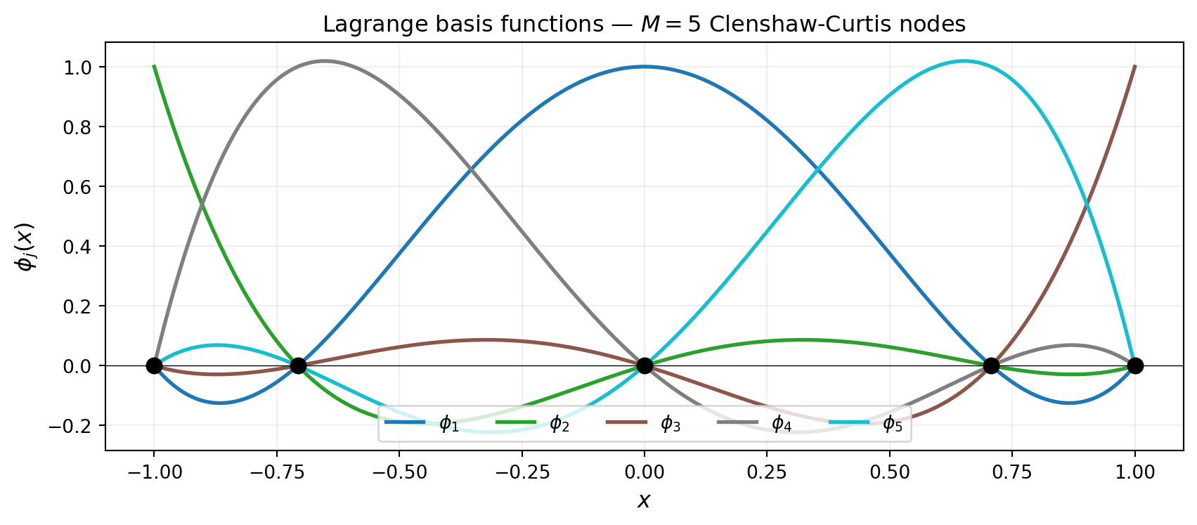
Using LagrangeBasis1D
LagrangeBasis1D takes a quadrature rule callable — any function with signature (npoints) → (samples, weights) — and builds the Lagrange basis at the rule’s nodes. This design lets us plug in Gauss, Clenshaw-Curtis, or Leja points interchangeably.
from pyapprox_tutorials.figures._interpolation import plot_basis_comparison

# --- Clenshaw-Curtis basis ---
cc_rule = ClenshawCurtisQuadratureRule(bkd, store=True)
basis_cc = LagrangeBasis1D(bkd, cc_rule)

M = 9  # CC requires 2^l + 1 points: 3, 5, 9, 17, ...
basis_cc.set_nterms(M)
nodes_cc, weights_cc = basis_cc.quadrature_rule()   # (1, M), (M, 1)

# --- Gauss-Legendre basis ---
poly = LegendrePolynomial1D(bkd)
poly.set_nterms(M)
gauss_rule = GaussQuadratureRule(poly, store=True)
basis_gauss = LagrangeBasis1D(bkd, gauss_rule)
basis_gauss.set_nterms(M)
nodes_gauss, weights_gauss = basis_gauss.quadrature_rule()

# Evaluate both bases on a fine grid
x_eval = bkd.array(np.linspace(-1, 1, 400).reshape(1, -1))
phi_cc    = bkd.to_numpy(basis_cc(x_eval))      # (400, 9)
phi_gauss = bkd.to_numpy(basis_gauss(x_eval))   # (400, 9)

x_plot = np.linspace(-1, 1, 400)
fig, axs = plt.subplots(1, 2, figsize=(13, 4), sharey=True)
plot_basis_comparison(
    x_plot, phi_cc, bkd.to_numpy(nodes_cc).ravel(),
    phi_gauss, bkd.to_numpy(nodes_gauss).ravel(), M, axs,
)
plt.suptitle("Lagrange basis functions — same $M$, different nodes", fontsize=12, y=1.02)
plt.tight_layout()
plt.show()
Both sets of basis functions satisfy \(\phi_j(x^{(k)}) = \delta_{jk}\), but their shapes differ because the nodes cluster differently. Clenshaw-Curtis nodes bunch up near \(\pm 1\) (Chebyshev distribution), while Gauss-Legendre nodes also cluster toward the endpoints but never include them.
The Runge Phenomenon
A natural first choice for interpolation nodes is equally spaced points. For \(M\) equally spaced nodes on \([-1, 1]\), the node product \(\prod_j |x - x^{(j)}|\) grows rapidly near the boundary as \(M\) increases, causing the interpolation error to diverge for many smooth functions. This failure mode is called the Runge phenomenon.
from pyapprox_tutorials.figures._interpolation import plot_runge

def runge(x):
    return 1.0 / (1.0 + 25.0 * x**2)


def lagrange_basis_manual(x, nodes):
    """Evaluate all M Lagrange basis functions at points x (manual formula)."""
    M = len(nodes)
    phi = np.ones((len(x), M))
    for j in range(M):
        for k in range(M):
            if k != j:
                phi[:, j] *= (x - nodes[k]) / (nodes[j] - nodes[k])
    return phi


M_equi = 13   # equidistant: any M works (manual formula)
M_cc   = 17   # CC requires 2^l + 1: 3, 5, 9, 17, ...
x_plot = np.linspace(-1, 1, 400)
true_vals = runge(x_plot)

# Equidistant nodes (manual — no pyapprox rule for these)
nodes_equi = np.linspace(-1, 1, M_equi)
interp_equi = lagrange_basis_manual(x_plot, nodes_equi) @ runge(nodes_equi)

# Clenshaw-Curtis nodes via pyapprox
basis_cc17 = LagrangeBasis1D(bkd, cc_rule)
basis_cc17.set_nterms(M_cc)
nodes_cc17, _ = basis_cc17.quadrature_rule()
nodes_cc_np = bkd.to_numpy(nodes_cc17).ravel()

x_eval = bkd.array(x_plot.reshape(1, -1))
phi_cc = bkd.to_numpy(basis_cc17(x_eval))   # (400, 17)
interp_cc = phi_cc @ runge(nodes_cc_np)

fig, axs = plt.subplots(1, 2, figsize=(13, 5), sharey=False)
plot_runge(x_plot, true_vals, nodes_equi, interp_equi, M_equi,
           nodes_cc_np, interp_cc, M_cc, axs)
plt.tight_layout()
plt.show()
The oscillations near \(\pm 1\) with equidistant nodes are not a numerical accident — they grow without bound as \(M \to \infty\) for Runge’s function. The cure is to cluster nodes toward the boundary, as both Clenshaw-Curtis and Gauss points do.
Clenshaw-Curtis Points
Clenshaw-Curtis (CC) nodes on \([-1, 1]\) are the Chebyshev points of the second kind:
\[ x^{(j)} = \cos\!\left(\frac{(j-1)\pi}{M-1}\right), \qquad j = 1, \ldots, M. \]
These are the projection of equally spaced points on the unit circle onto the real axis. They minimise \(\max_{x \in [-1,1]} \prod_j |x - x^{(j)}|\) among all \(M\)-point sets with endpoints fixed at \(\pm 1\), making them near-optimal for interpolation.
A critical property for sparse grids is that CC nodes are nested: the \(M = 2^k + 1\) point CC grid contains all points of the \(M = 2^{k-1} + 1\) point grid.
from pyapprox_tutorials.figures._interpolation import plot_nested_cc

levels = [3, 5, 9]

fig, ax = plt.subplots(figsize=(10, 3))
plot_nested_cc(cc_rule, bkd, levels, ax)
plt.tight_layout()
plt.show()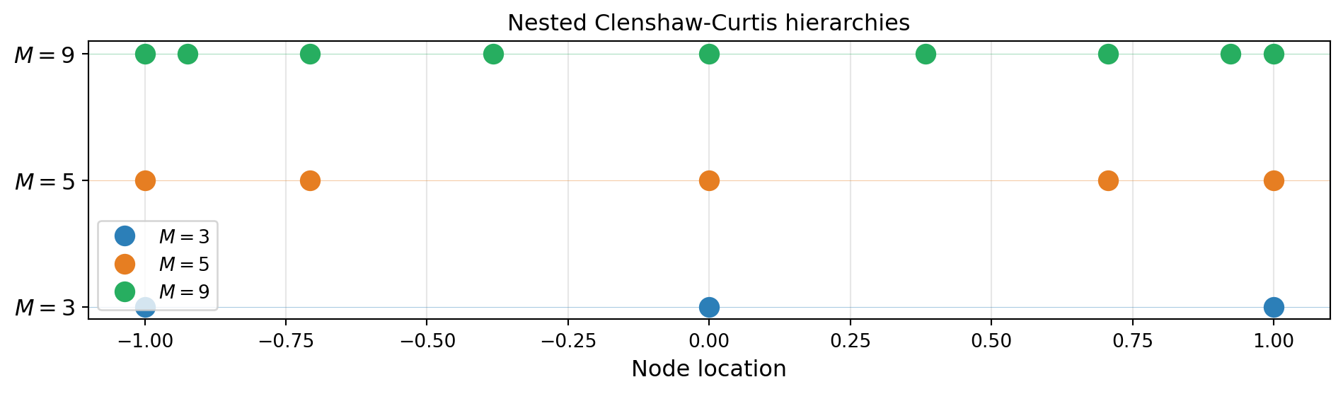
Convergence Study
For a function with \(r\) continuous derivatives, the Lagrange interpolant on Chebyshev-type nodes converges at rate \(O(M^{-r})\). For analytic functions (smooth everywhere in the complex plane) the convergence is exponential: \(O(\rho^{-M})\) for some \(\rho > 1\).
from pyapprox_tutorials.figures._interpolation import plot_interp_convergence

def f_analytic(x):
    return np.exp(np.cos(np.pi * x))

def f_c1(x):
    return np.abs(x) * np.maximum(x, 0)   # C^1, not C^2

test_funcs = [
    (f_analytic, r"$e^{\cos(\pi x)}$ — analytic"),
    (runge,      r"$1/(1+25x^2)$ — analytic"),
    (f_c1,       r"$x\max(x,0)$ — $C^1$ only"),
]

x_ref = np.linspace(-1, 1, 2000)
Ms = [3, 5, 9, 17]

x_eval = bkd.array(x_ref.reshape(1, -1))

errors_by_func = []
labels = []
for func, label in test_funcs:
    true_vals_ref = func(x_ref)
    errors = []
    for M in Ms:
        basis_M = LagrangeBasis1D(bkd, cc_rule)
        basis_M.set_nterms(M)
        nodes_M, _ = basis_M.quadrature_rule()
        nodes_M_np = bkd.to_numpy(nodes_M).ravel()
        phi_M = bkd.to_numpy(basis_M(x_eval))   # (2000, M)
        interp_vals = phi_M @ func(nodes_M_np)
        errors.append(np.max(np.abs(true_vals_ref - interp_vals)))
    errors_by_func.append(errors)
    labels.append(label)

fig, ax = plt.subplots(figsize=(9, 5))
plot_interp_convergence(Ms, errors_by_func, labels, ax)
plt.tight_layout()
plt.show()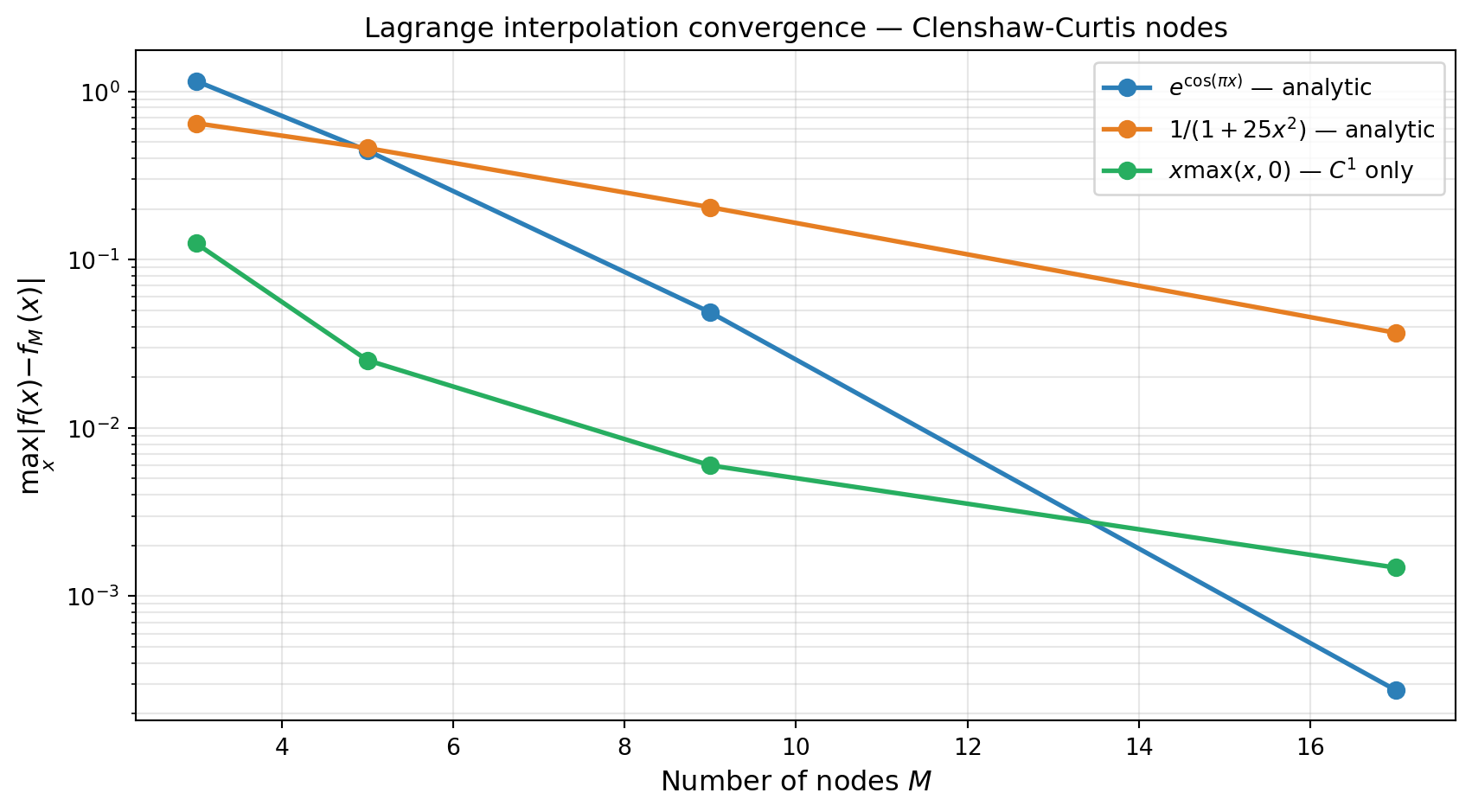
Both analytic test functions converge exponentially (straight lines on the semi-log plot). The \(C^1\) function converges algebraically, consistent with the theoretical rate \(O(M^{-2})\).
Interpolation Weights as Quadrature Weights
Integrating the interpolant \(f_M(x) = \sum_j f(x^{(j)}) \phi_j(x)\) over \([a, b]\) gives
\[ \int_a^b f_M(x)\, dx = \sum_{j=1}^{M} f\!\left(x^{(j)}\right) \underbrace{\int_a^b \phi_j(x)\, dx}_{=:\, w_j}. \]
The quadrature weights \(w_j\) are exactly the integrals of the Lagrange basis functions. This means that any quadrature rule based on Lagrange interpolation (Gauss, Clenshaw-Curtis, and many others) can be recovered by integrating the basis polynomials analytically.
# Verify: CC quadrature weights via basis integration agree with the rule's weights.
M = 5
basis_verify = LagrangeBasis1D(bkd, cc_rule)
basis_verify.set_nterms(M)
_, rule_weights = basis_verify.quadrature_rule()  # (M, 1)
rule_w_np = bkd.to_numpy(rule_weights).ravel()

# Compute weights by integrating each basis polynomial on [-1, 1]
x_fine = np.linspace(-1, 1, 10_000)
x_fine_bkd = bkd.array(x_fine.reshape(1, -1))
phi_fine = bkd.to_numpy(basis_verify(x_fine_bkd))  # (10000, M)

# Integrate with probability measure (divide by 2 for [-1,1])
computed_weights = np.trapezoid(phi_fine, x_fine, axis=0) / 2.0
The weights from integrating the Lagrange basis functions (divided by 2 to convert from Lebesgue to probability measure) match the Clenshaw-Curtis quadrature weights to high precision.
Key Takeaways
- Lagrange interpolants pass through every data point by construction; the interpolation property \(\phi_j(x^{(k)}) = \delta_{jk}\) makes the coefficients simply the function values at the nodes.
- Equidistant nodes cause the Runge phenomenon — interpolation error can grow without bound for smooth functions. Chebyshev-type nodes (Clenshaw-Curtis, Gauss) eliminate this by clustering nodes toward the boundary.
- Clenshaw-Curtis nodes are nested across the hierarchy \(M = 3, 5, 9, 17, \ldots\), which is essential for the sparse grid construction in later tutorials.
- The quadrature weights of any interpolation-based rule are the integrals of the corresponding Lagrange basis functions.
Exercises
NoteExercises
Basis functions. Plot the Lagrange basis \(\phi_j\) for \(M = 9\) equidistant nodes. How large can \(|\phi_j(x)|\) get between nodes? Compare with CC nodes of the same size.
Runge revisited. Find the smallest \(M\) such that the equidistant interpolant of \(1/(1+25x^2)\) has maximum error below \(0.5\). How does this compare to the CC result?
Convergence rate. For \(f(x) = |x|^{2.5}\) (which is \(C^2\) but not \(C^3\)), what algebraic convergence rate do you observe? Does the theoretical rate \(O(M^{-3})\) match?
Quadrature accuracy. Use the CC nodes to integrate \(f(x) = e^x\) on \([-1, 1]\) for \(M = 3, 5, 9, 17\). At what \(M\) do you reach machine precision? Compare with \(M\)-point Gauss–Legendre.
Next Steps
- Leja Sequences: Nested Points for Adaptive Interpolation — A greedy alternative to CC for non-uniform distributions
- Piecewise Polynomial Interpolation — Local basis functions that handle discontinuous functions gracefully