GP-Based Sensitivity Analysis

PyApprox Tutorial Library

Computing Sobol indices analytically from GP kernel integrals and verifying against fix-and-freeze estimates.

TipDownload Notebook

Download as Jupyter Notebook

Learning Objectives

After completing this tutorial, you will be able to:

• Use GaussianProcessSensitivity to compute Sobol indices from kernel integrals
• Explain how conditional variances from the GP posterior yield Sobol indices
• Verify GP-based indices against sample-based fix-and-freeze (Saltelli/Jansen) estimates
• Assess accuracy by comparing both methods against known analytical ground truth

Prerequisites

Complete:

• Sensitivity Analysis — variance decomposition and Sobol index definitions
• Building a GP Surrogate — GP fitting basics

How GP Sensitivity Analysis Works

Why a separable kernel?

All the GP-based UQ and sensitivity formulas require integrating the kernel function over the input distribution \(\rho(\boldsymbol{\xi})\). A generic \(D\)-dimensional kernel integral

\[ \int k(\boldsymbol{\xi}, \boldsymbol{\xi}^{(i)})\, \rho(\boldsymbol{\xi})\,\dd\boldsymbol{\xi} \]

would require \(D\)-dimensional quadrature, which is intractable for even moderate \(D\). With a separable product kernel \(k(\boldsymbol{\xi}, \boldsymbol{\xi}') = \prod_{d=1}^{D} k_d(\xi_d, \xi_d')\) and independent marginals \(\rho = \prod_d \rho_d\), this integral factors into a product of \(D\) cheap one-dimensional integrals:

\[ \int k(\boldsymbol{\xi}, \boldsymbol{\xi}^{(i)})\,\rho(\boldsymbol{\xi})\,\dd\boldsymbol{\xi} = \prod_{d=1}^{D} \int k_d(\xi_d, \xi_d^{(i)})\,\rho_d(\xi_d)\,\dd\xi_d \]

Each 1D integral is computed to machine precision with a small Gauss quadrature rule (e.g., 20–30 points). This factorisation is the sole reason a separable kernel is required: it turns intractable multivariate integrals into products of 1D quadrature sums.

From conditional variances to Sobol indices

For a GP with posterior mean \(\mu^*(\boldsymbol{\xi})\) and posterior variance \(\gamma_f(\boldsymbol{\xi}) = \sigma^{*2}(\boldsymbol{\xi})\) (the GP’s pointwise uncertainty about the true function value), Sobol indices can be computed analytically by integrating conditional variances over the input distribution.

The key idea is that the conditional variance — the variance of the GP mean when a subset of inputs \(\boldsymbol{\xi}_p\) is held fixed and the remaining inputs are integrated out — equals the ANOVA variance component for that subset:

\[ V_p = \E_{\boldsymbol{\xi}_{\sim p}}\bigl[ \Var_{\boldsymbol{\xi}_p}[\mu^*(\boldsymbol{\xi}) \mid \boldsymbol{\xi}_{\sim p}] \bigr] = \boldsymbol{\alpha}^\top P_p \boldsymbol{\alpha} - (\boldsymbol{\tau}^\top \boldsymbol{\alpha})^2 \]

where \(P_p\) is the conditional P matrix: for dimensions in \(p\) the entries are kernel evaluations at the training points, while for the remaining dimensions the kernel is integrated against \(\rho\). Thanks to separability, \(P_p\) factors into products of 1D integrals — each either a kernel evaluation or a 1D quadrature sum — so the entire matrix is cheap to assemble.

The first-order and total-effect Sobol indices are then:

\[ \Sobol{i} = \frac{V_{\{i\}}}{\Var_{\boldsymbol{\xi}}[\mu^*(\boldsymbol{\xi})]}, \qquad \SobolT{i} = 1 - \frac{V_{\sim\{i\}}}{\Var_{\boldsymbol{\xi}}[\mu^*(\boldsymbol{\xi})]} \]

where \(V_{\{i\}}\) conditions on variable \(i\) alone, \(V_{\sim\{i\}}\) conditions on all variables except \(i\), and \(\Var_{\boldsymbol{\xi}}[\mu^*(\boldsymbol{\xi})]\) is the total variance of the GP posterior mean under the input distribution.

Setup

We use the Ishigami benchmark, a standard 3-variable test function with known analytical Sobol indices:

\[ f(x_1, x_2, x_3) = \sin(x_1) + 7\sin^2(x_2) + 0.1\, x_3^4 \sin(x_1) \]

import numpy as np
import matplotlib.pyplot as plt
from pyapprox.util.backends.numpy import NumpyBkd
from pyapprox.benchmarks import ishigami_3d
from pyapprox.surrogates.gaussianprocess import ExactGaussianProcess
from pyapprox.surrogates.kernels.composition import SeparableProductKernel
from pyapprox.surrogates.kernels.matern import SquaredExponentialKernel
from pyapprox.surrogates.gaussianprocess.fitters import (
    GPMaximumLikelihoodFitter,
)

bkd = NumpyBkd()
np.random.seed(42)

# Load benchmark
benchmark = ishigami_3d(bkd)
func = benchmark.function()
prior = benchmark.prior()
gt = benchmark.ground_truth()
marginals = prior.marginals()
nvars = 3

gt_main = bkd.to_numpy(gt.main_effects).flatten()
gt_total = bkd.to_numpy(gt.total_effects).flatten()

ImportantSeparable kernel required

As explained above, the analytical formulas require a separable product kernel so that all multivariate kernel integrals reduce to products of 1D Gauss quadrature sums. We use a SeparableProductKernel composed of independent 1D squared-exponential kernels, one per input dimension.

# Fit GP with separable SE kernel
kernels = [
    SquaredExponentialKernel([1.0], (0.01, 20.0), 1, bkd)
    for _ in range(nvars)
]
kernel = SeparableProductKernel(kernels, bkd)
gp = ExactGaussianProcess(kernel, nvars=nvars, bkd=bkd, nugget=1e-8)

N_train = 1500
X_train = prior.rvs(N_train)
y_train = func(X_train)

fitter = GPMaximumLikelihoodFitter(bkd)
result = fitter.fit(gp, X_train, y_train)
gp = result.surrogate()

# Verify accuracy
np.random.seed(123)
X_test = prior.rvs(2000)
y_test = func(X_test)
y_pred = gp.predict(X_test)
rel_rmse = float(bkd.to_numpy(
    bkd.sqrt(bkd.mean((y_test - y_pred)**2)) / bkd.sqrt(bkd.mean(y_test**2))
))

GP Kernel-Integral Sobol Indices

The GaussianProcessSensitivity class wraps a GaussianProcessStatistics object and computes Sobol indices from the conditional P matrices described above.

from pyapprox.surrogates.sparsegrids.basis_factory import (
    create_basis_factories,
)
from pyapprox.surrogates.gaussianprocess.statistics import (
    SeparableKernelIntegralCalculator,
    GaussianProcessStatistics,
    GaussianProcessSensitivity,
)

# Build integral calculator with Gauss-Legendre quadrature (uniform inputs)
nquad = 30
factories = create_basis_factories(marginals, bkd, "gauss")
bases = [f.create_basis() for f in factories]
for b in bases:
    b.set_nterms(nquad)

calc = SeparableKernelIntegralCalculator(gp, bases, marginals, bkd=bkd)
stats = GaussianProcessStatistics(gp, calc)
sens = GaussianProcessSensitivity(stats)

# Main effects (first-order indices)
main_effects_gp = sens.main_effect_indices()   # Dict[int, Array]
total_effects_gp = sens.total_effect_indices()  # Dict[int, Array]

S1_gp = np.array([float(bkd.to_numpy(main_effects_gp[d])) for d in range(nvars)])
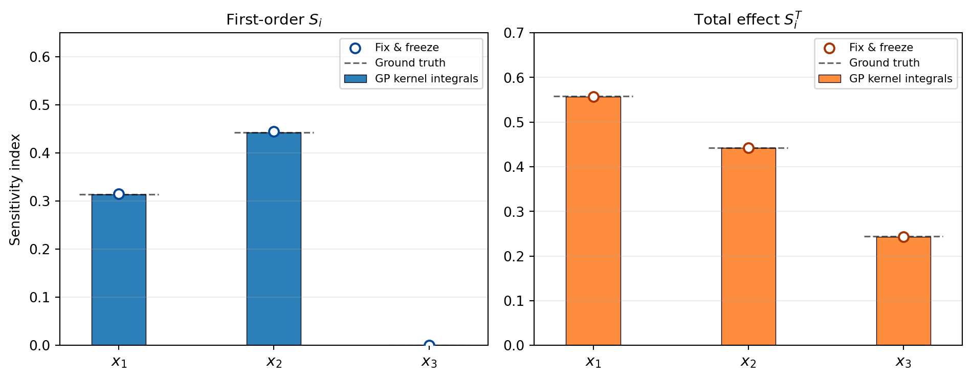
ST_gp = np.array([float(bkd.to_numpy(total_effects_gp[d])) for d in range(nvars)])

Note that \(\Sobol{3} \approx 0\) (no main effect for \(x_3\)) but \(\SobolT{3} > 0\) (due to the \(x_1 x_3\) interaction term \(0.1\,x_3^4\sin(x_1)\)).

Fix-and-Freeze Verification

As an independent check, we compute Sobol indices via the Saltelli/Jansen fix-and-freeze estimator, evaluating the GP surrogate at the Saltelli sample matrices. Since the GP is cheap to evaluate, this uses the surrogate in place of the true model.

from pyapprox.sensitivity import SobolSequenceSensitivityAnalysis

sa = SobolSequenceSensitivityAnalysis(prior, bkd, seed=42)
sa_samples = sa.generate_samples(8192)       # (nvars, 8192*(2+nvars))
sa_values = gp.predict(sa_samples)           # (1, nsamples_total)
sa.compute(sa_values)

S1_ff = bkd.to_numpy(sa.main_effects())[:, 0]
ST_ff = bkd.to_numpy(sa.total_effects())[:, 0]

Comparison

Both methods — GP kernel integrals and fix-and-freeze — agree closely with the known analytical values. Figure 1 shows both estimates side-by-side.

Figure 1: GP-based Sobol indices for the Ishigami function. Bars show GP kernel-integral estimates; dots show fix-and-freeze (Saltelli/Jansen) estimates; dashed lines mark the analytical ground truth.

Variability of GP Sobol Indices

The kernel-integral formulas above give point estimates \(\Sobol{i} = V_{\{i\}} / \Var_{\boldsymbol{\xi}}[\mu^*]\). But the GP posterior is uncertain about the true function, so the Sobol indices themselves are random variables. How much would \(\Sobol{i}\) change if we drew a different function from the GP posterior?

Ensemble approach

The GaussianProcessEnsemble class answers this question by sampling GP realizations and computing Sobol indices for each one:

1. Draw \(R\) function realizations from the GP posterior using the reparameterization trick: \[ f^{(r)}(\boldsymbol{\xi}) = \mu^*(\boldsymbol{\xi}) + L\,\boldsymbol{\varepsilon}^{(r)}, \qquad \boldsymbol{\varepsilon}^{(r)} \sim \mathcal{N}(\mathbf{0}, I) \] where \(L\) is the Cholesky factor of the posterior covariance \(\Sigma^* = k(\boldsymbol{\xi}, \boldsymbol{\xi}') - \mathbf{k}^{*\top} K^{-1} \mathbf{k}^*\) evaluated at a set of Monte Carlo integration points.

2. For each realization \(r\), estimate the total variance and conditional variances by Monte Carlo integration: \[ \gamma_f^{(r)} = \int [f^{(r)}]^2\,\rho\,\dd\boldsymbol{\xi} - \Bigl(\int f^{(r)}\,\rho\,\dd\boldsymbol{\xi}\Bigr)^2, \qquad V_i^{(r)} = \Var_{\xi_i}\!\bigl[\E_{\boldsymbol{\xi}_{\sim i}}[f^{(r)} \mid \xi_i]\bigr] \]

3. Compute the Sobol index for each realization: \(\Sobol{i}^{(r)} = V_i^{(r)} / \gamma_f^{(r)}\).

The empirical distribution of \(\{\Sobol{i}^{(r)}\}_{r=1}^{R}\) gives the mean, standard deviation, and confidence intervals for each Sobol index.

NoteWhy not use the analytical point estimate directly?

The analytical formula computes \(\E[\Sobol{i}]\) only approximately, because \(\Sobol{i} = V_i / \gamma_f\) is a ratio of random variables and \(\E[V_i / \gamma_f] \neq \E[V_i] / \E[\gamma_f]\) (Jensen’s inequality). The ensemble approach evaluates the ratio for each realization, correctly capturing the full distribution including any skewness.

from pyapprox.surrogates.gaussianprocess.statistics import (
    GaussianProcessEnsemble,
)

ensemble = GaussianProcessEnsemble(gp, sens)
S_dist = ensemble.compute_sobol_distribution(
    n_realizations=500,
    n_sample_points=800,
    seed=42,
)

from pyapprox.tutorial_figures._gp import plot_sobol_distribution

fig, axes = plt.subplots(1, nvars, figsize=(12, 3.5), sharey=True)
plot_sobol_distribution(axes, nvars, S_dist, gt_main, bkd)
plt.suptitle("GP posterior uncertainty in Sobol indices", fontsize=11, y=1.02)
plt.tight_layout()
plt.show()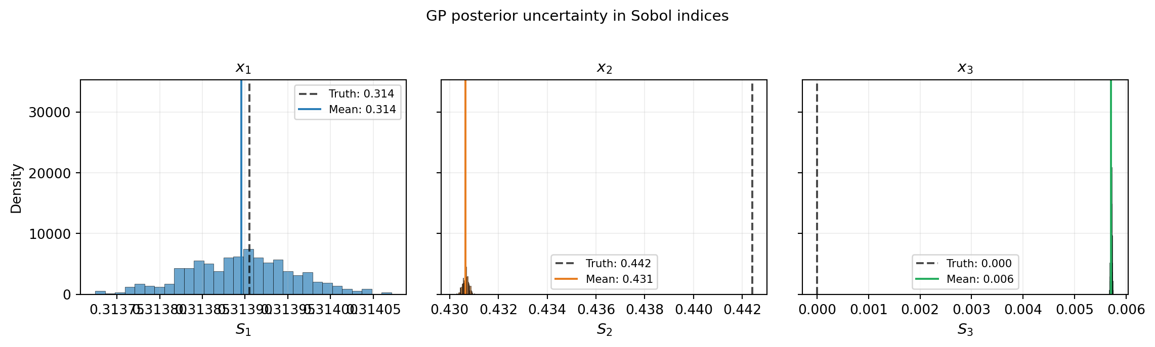

Figure 2: Distribution of first-order Sobol indices across 500 GP posterior realizations. Histograms show the spread due to GP uncertainty; vertical dashed lines mark the analytical ground truth. Narrow distributions indicate the GP has enough training data to pin down the sensitivity structure.

Key Takeaways

• GaussianProcessSensitivity computes Sobol indices analytically from GP kernel integrals — no additional sampling needed beyond the training data
• The method requires a separable product kernel so that all multivariate kernel integrals reduce to products of cheap 1D quadrature sums
• GP kernel-integral indices agree closely with sample-based fix-and-freeze estimates, confirming the analytical formulas are correctly implemented
• GaussianProcessEnsemble quantifies the uncertainty in the Sobol indices themselves by sampling GP realizations and computing the index distribution
• Like PCE-based sensitivity, index accuracy depends on how well the GP approximates the true function

Exercises

1. (Easy) Reduce the training set from \(N=1500\) to \(N=200\). How do the GP-based Sobol indices change? Are the fix-and-freeze estimates more or less robust to the reduced GP accuracy?

2. (Medium) Use sens.conditional_variance(index) directly to compute the second-order interaction index \(\Sobol{13}\). Verify it matches the known value \(S_{13} \approx 0.244\).

3. (Challenge) Compare the GP sensitivity results against PCE-based sensitivity for the same Ishigami function (see PCE Sensitivity). Which surrogate needs fewer training points to achieve accurate Sobol indices?

Next Steps

• PCE-Based Sensitivity — Analogous Sobol analysis from polynomial chaos expansion coefficients
• UQ with Gaussian Processes — Analytical moments and marginal densities from GP kernel integrals
• Morris Screening — Cheap screening to identify important inputs before Sobol analysis