import numpy as np
import matplotlib.pyplot as plt
import torch
torch.set_default_dtype(torch.float64)

from pyapprox.util.backends.torch import TorchBkd
from pyapprox_benchmarks.statest import (
    ForresterEnsembleProblem,
)

bkd = TorchBkd()
bench = ForresterEnsembleProblem(bkd)
models = bench.problem().models()          # [HF model, LF model]
prior = bench.problem().prior()
nvars = 1
nmodels = 2

# Reorder so level 0 = LF (cheap), level 1 = HF (expensive)
level_models = [models[1], models[0]]
level_names = ["Low fidelity", "High fidelity"]
costs_per_eval = [0.05, 1.0] # seconds per evaluationMulti-Fidelity Gaussian Processes
PyApprox Tutorial Library
Exploit correlations between model fidelities to build accurate surrogates within a fixed computational budget.
TipDownload Notebook
Learning Objectives
After completing this tutorial you will be able to:
- Build a
MultiLevelKernelfrom per-level kernels and aPolynomialScalingFunctioncorrelation function to represent the Kennedy–O’Hagan auto-regressive model - Fit and predict with
TorchMultiOutputGP, including predictive uncertainty bands - Compare multi-fidelity and single-fidelity GP surrogates at equal computational budget
- Interpret the block kernel matrix that encodes inter-level correlations
The Multi-Fidelity Idea
Many simulators exist at multiple fidelity levels: a cheap approximation captures the broad trend while an expensive high-fidelity model adds fine-scale detail. The outputs are highly correlated — the cheap model is inaccurate in absolute terms but tracks the expensive model closely enough to carry information.
A multi-fidelity Gaussian process (MFGP) models this relationship explicitly, so that many cheap evaluations substantially reduce uncertainty in the high-fidelity prediction. The accuracy gain is largest when the cost ratio is high and the inter-level correlation is strong.
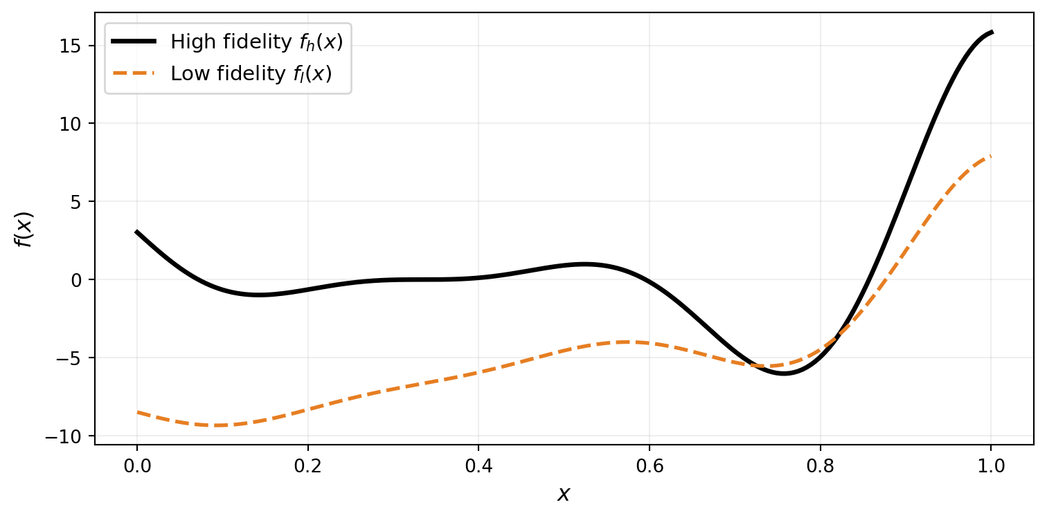
Setup: The Forrester Benchmark
We use the Forrester multi-fidelity benchmark — a pair of 1D functions sharing the same oscillatory structure but differing in scale and offset. The high-fidelity function \(f_h(x) = (6x - 2)^2 \sin(12x - 4)\) is expensive; the low-fidelity approximation \(f_l(x) = 0.5\, f_h(x) + 10(x - 0.5) - 5\) is cheap but biased.
The Kennedy–O’Hagan Auto-Regressive Model
The MFGP is built on the Kennedy–O’Hagan (KO) model, which relates each fidelity level \(k\) to the level below through a scaling and an independent discrepancy GP:
\[ f_0 \sim \mathcal{GP}(0, k_0), \qquad f_k = \rho_{k-1}\,f_{k-1} + \delta_k, \quad k = 1, \ldots, K-1 \]
where \(\rho_{k-1}\) is a scaling constant and \(\delta_k \sim \mathcal{GP}(0, k_k)\) is an independent discrepancy. Recursively expanding this expression yields the joint covariance across all levels — a block matrix that MultiLevelKernel assembles automatically.
For the Forrester benchmark, the true relationship is \(f_h = 2\, f_l + \text{offset}\), so the optimal scaling is \(\rho \approx 2\).
Building the MultiLevelKernel
from pyapprox.surrogates.kernels.matern import SquaredExponentialKernel
from pyapprox.surrogates.kernels.multioutput.multilevel import MultiLevelKernel
from pyapprox.surrogates.kernels.scalings import PolynomialScalingFunction
from pyapprox.surrogates.gaussianprocess.torch_multioutput import TorchMultiOutputGP

# One SE kernel per fidelity level (the k_k terms in the KO model)
level_kernels = [
    SquaredExponentialKernel([1.0], (0.01, 10.0), nvars, bkd)
    for _ in range(nmodels)
]

# Scaling function for the LF -> HF transition.
# We fix rho = 2.0 (the known Forrester relationship) and only
# optimise the correlation length scales via MLL.
scalings = [
    PolynomialScalingFunction([2.0], (-5.0, 5.0), bkd, nvars=nvars, fixed=True),
]

mf_kernel = MultiLevelKernel(level_kernels, scalings)

# TorchMultiOutputGP uses autograd to differentiate the NLL directly,
# bypassing the kernel's analytical jacobian_wrt_params.
mf_gp = TorchMultiOutputGP(mf_kernel, nugget=1e-6)
NoteFixing vs. learning the scaling
For the Forrester benchmark we fix \(\rho = 2\) because the analytical relationship is known. In practice, \(\rho\) can be estimated from a small pilot study or learned jointly with the length scales by setting fixed=False. Learning \(\rho\) via MLL can be sensitive to local optima, especially for highly oscillatory functions with few high-fidelity samples.
Training Data
We allocate 100 cheap low-fidelity evaluations and only 4 expensive high-fidelity evaluations. The total cost is \(100 \times 0.05 + 4 \times 1.0 = 9\) seconds — equivalent to 9 high-fidelity evaluations.
n_lf, n_hf = 100, 4
np.random.seed(42)
X_lf = prior.rvs(n_lf)
X_hf = prior.rvs(n_hf)
y_lf = level_models[0](X_lf)     # shape (1, n_lf)
y_hf = level_models[1](X_hf)     # shape (1, n_hf)

samples_list = [X_lf, X_hf]
y_train_list = [y_lf, y_hf]

total_cost = n_lf * costs_per_eval[0] + n_hf * costs_per_eval[1]
Fitting and Predicting
from pyapprox.surrogates.gaussianprocess.fitters import MultiOutputGPMaximumLikelihoodFitter

# fit() optimises all active hyperparameters (length scales) via MLL
result = MultiOutputGPMaximumLikelihoodFitter(bkd).fit(
    mf_gp, samples_list, y_train_list
)
mf_gp = result.surrogate()

# Predict on a dense grid with uncertainty
x_test = bkd.asarray(np.linspace(0, 1, 200).reshape(1, -1))
X_test_list = [x_test] * nmodels
means, stds = mf_gp.predict_with_uncertainty(X_test_list)

mf_pred = bkd.to_numpy(means[-1])[0, :]      # HF-level mean
mf_std = bkd.to_numpy(stds[-1])[0, :]         # HF-level std

y_test_hf = bkd.to_numpy(level_models[1](x_test))[0, :]
l2_mf = np.linalg.norm(y_test_hf - mf_pred) / np.linalg.norm(y_test_hf)
HF-Only Baseline
For a fair comparison, we build a single-fidelity GP using the same total computational budget spent entirely on high-fidelity evaluations.
from pyapprox.surrogates.gaussianprocess import ExactGaussianProcess
from pyapprox.surrogates.gaussianprocess.fitters import (
    GPMaximumLikelihoodFitter,
)

n_hf_equiv = int(total_cost / costs_per_eval[-1])   # 9 HF evals
np.random.seed(7)
X_hf_only = prior.rvs(n_hf_equiv)
y_hf_only = level_models[-1](X_hf_only)

hf_kern = SquaredExponentialKernel([1.0], (0.01, 10.0), nvars, bkd)
hf_gp = ExactGaussianProcess(hf_kern, nvars=nvars, bkd=bkd, nugget=1e-6)
hf_gp = GPMaximumLikelihoodFitter(bkd).fit(
    hf_gp, X_hf_only, y_hf_only
).surrogate()

hf_pred = bkd.to_numpy(hf_gp.predict(x_test))[0, :]
hf_std = bkd.to_numpy(hf_gp.predict_std(x_test))[0, :]
l2_hf = np.linalg.norm(y_test_hf - hf_pred) / np.linalg.norm(y_test_hf)

# HF-only baseline using the SAME 4 HF samples as the MF GP
hf_kern_few = SquaredExponentialKernel([1.0], (0.01, 10.0), nvars, bkd)
hf_gp_few = ExactGaussianProcess(hf_kern_few, nvars=nvars, bkd=bkd, nugget=1e-6)
hf_gp_few = GPMaximumLikelihoodFitter(bkd).fit(
    hf_gp_few, X_hf, y_hf
).surrogate()
hf_few_pred = bkd.to_numpy(hf_gp_few.predict(x_test))[0, :]
hf_few_std = bkd.to_numpy(hf_gp_few.predict_std(x_test))[0, :]
l2_hf_few = np.linalg.norm(y_test_hf - hf_few_pred) / np.linalg.norm(y_test_hf)
Comparison: Predictions and Uncertainty

The Block Kernel Matrix
The MultiLevelKernel assembles a joint covariance across all fidelity levels. Off-diagonal blocks encode the cross-level correlations implied by the KO recursion: large values mean a low-fidelity evaluation carries information about the high-fidelity level.

NoteReading the kernel heatmap
Each diagonal block is the per-level prior covariance. The off-diagonal blocks are cross-level covariances implied by the KO recursion: a large LF–HF block means a low-fidelity evaluation carries significant information about the high-fidelity level. The scaling \(\rho = 2\) amplifies this cross-level covariance, which is why 100 cheap LF evaluations so effectively reduce uncertainty in the HF prediction.
Key Takeaways
- The Kennedy–O’Hagan model \(f_k = \rho_{k-1}\,f_{k-1} + \delta_k\) encodes inter-level correlation explicitly;
MultiLevelKernelassembles the block kernel matrix automatically from per-level kernels and scalings - Fixing \(\rho\) to a known or estimated value avoids local-optima issues in MLL optimisation; the GP then learns only the correlation length scales
- The multi-fidelity GP achieves tighter uncertainty bands and lower prediction error by transferring information from cheap low-fidelity evaluations
- The block kernel matrix visualises how much information flows between levels
Exercises
- Set \(\rho = 0.5\) (fixed) and refit. How does the HF prediction quality change? What does this tell you about the sensitivity to the scaling value?
- Set
fixed=Falseon thePolynomialScalingFunctionto let the GP learn \(\rho\). Does it recover \(\rho \approx 2\)? If not, try increasing the nugget to1e-4— does this help the optimiser find a better minimum? - Reduce the number of LF evaluations from 100 to 20 while keeping 4 HF. At what LF sample size does the multi-fidelity advantage disappear?
Next Steps
- Gaussian Process Surrogates — Single-output GP fundamentals including kernel selection and MLL fitting
- UQ with Gaussian Processes — Using GP surrogates for uncertainty quantification tasks