import numpy as np
import matplotlib.pyplot as plt
from pyapprox.util.backends.numpy import NumpyBkd
from pyapprox_benchmarks.pde.cantilever_beam import (
    build_cantilever_beam_1d,
)
from pyapprox.surrogates.affine.expansions.pce import (
    create_pce_from_marginals,
)
from pyapprox.surrogates.affine.expansions.fitters.least_squares import (
    LeastSquaresFitter,
)

bkd = NumpyBkd()

problem = build_cantilever_beam_1d(bkd, num_kle_terms=3)
model = problem.function()
prior = problem.prior()
marginals = prior.marginals()
nvars = model.nvars()
nqoi = model.nqoi()

qoi_labels = [
    r"$\delta_{\mathrm{tip}}$",
    r"$\sigma_{\mathrm{int}}$",
    r"$\kappa_{\max}$",
]

# Training data
N_train = 100
np.random.seed(42)
samples_train = prior.rvs(N_train)
values_train = model(samples_train)

# Fit degree-3 PCE
degree = 3
pce = create_pce_from_marginals(marginals, degree, bkd, nqoi=nqoi)
ls_fitter = LeastSquaresFitter(bkd)
pce = ls_fitter.fit(pce, samples_train, values_train).surrogate()UQ with Polynomial Chaos
PyApprox Tutorial Library
Extract analytical moments, marginal densities, and convergence comparisons from a fitted PCE.
TipDownload Notebook
Learning Objectives
After completing this tutorial, you will be able to:
- Compute the mean, variance, and covariance of QoIs analytically from PCE coefficients
- Explain why orthonormality makes these moment formulas exact
- Sample a fitted surrogate to estimate marginal densities of the QoIs
- Use PCE marginalization to visualize main effect functions and pairwise input interactions
- Compare PCE-based and Monte Carlo moment estimates at the same computational budget
Prerequisites
Complete Building a Polynomial Chaos Surrogate before this tutorial.
Setup: Fit a PCE
We use a 1D Euler–Bernoulli cantilever beam with spatially varying bending stiffness \(EI(x)\) parameterized by a 3-term Karhunen–Lo`eve expansion. The three KLE coefficients \(\xi_1, \xi_2, \xi_3 \sim \mathcal{N}(0,1)\) are the uncertain inputs. The model returns three QoIs: tip deflection, integrated bending stress, and maximum curvature.
Analytical Moments from PCE Coefficients
The orthonormality of the PCE basis,
\[ \mathbb{E}[\Psi_i(\boldsymbol{\theta})\, \Psi_j(\boldsymbol{\theta})] = \delta_{ij}, \]
gives us the mean, variance, and covariance of the QoIs for free — no additional model evaluations, no sampling, no numerical integration:
\[ \mathbb{E}[f_k] = c_{0,k}, \qquad \text{Var}[f_k] = \sum_{j=1}^{P-1} c_{j,k}^2, \qquad \text{Cov}[f_j, f_k] = \sum_{i=1}^{P-1} c_{i,j}\, c_{i,k} \]
The mean is the zeroth coefficient (constant term), and the variance is the sum of squares of all other coefficients. Once the PCE is fitted, moment computation is instantaneous.
pce_mean = bkd.to_numpy(pce.mean())           # (nqoi,)
pce_var = bkd.to_numpy(pce.variance())         # (nqoi,)
pce_cov = bkd.to_numpy(pce.covariance())       # (nqoi, nqoi)
ImportantWhy are these exact?
These formulas are not approximations — they are exact for the fitted PCE. They compute the moments of the surrogate \(\hat{f}\), not of the true model \(f\). The only source of error is the surrogate approximation itself.
Marginal Densities: Fair Cost Comparison
To compare the PCE surrogate against direct Monte Carlo fairly, both approaches must use the same total wall-clock budget. We use timed() to measure the mean execution time per evaluation of the beam model and the PCE, then allocate budgets so the total cost is equivalent to 500 beam evaluations:
\[ N_{\text{train}} \times t_{\text{beam}} + M \times t_{\text{PCE}} = 500 \times t_{\text{beam}} \quad\Longrightarrow\quad M = \frac{(500 - N_{\text{train}}) \times t_{\text{beam}}}{t_{\text{PCE}}} \]
from pyapprox.interface.functions.timing import timed
from pyapprox_tutorials.figures._pce import plot_pce_marginal_densities

# Measure per-evaluation cost of beam model and PCE
timed_model = timed(model)
np.random.seed(0)
warmup_samples = prior.rvs(50)
_ = timed_model(warmup_samples)
beam_cost = timed_model.timer().get("__call__").median()

timed_pce = timed(pce)
_ = timed_pce(warmup_samples)
pce_cost = timed_pce.timer().get("__call__").median()

# Equal-cost sample sizes
N_mc = 500
M_pce = int((N_mc - N_train) * beam_cost / pce_cost)

# MC reference: 500 beam evaluations
np.random.seed(123)
samples_mc = prior.rvs(N_mc)
vals_mc = bkd.to_numpy(model(samples_mc))  # (nqoi, N_mc)

# PCE: M_pce equivalent-cost surrogate evaluations
np.random.seed(99)
samples_pce = prior.rvs(M_pce)
preds_pce = bkd.to_numpy(pce(samples_pce))  # (nqoi, M_pce)

fig, axes = plt.subplots(1, nqoi, figsize=(14, 4))
plot_pce_marginal_densities(vals_mc, preds_pce, N_mc, N_train, M_pce,
                            qoi_labels, axes)
plt.tight_layout()
plt.show()
The PCE produces much smoother density estimates because the surrogate is orders of magnitude cheaper than the beam model. At equal wall-clock cost, the PCE can draw \(M \gg 500\) samples, while MC is limited to 500 noisy evaluations.
Marginal Plots via PCE Marginalization
PCE orthonormality makes input marginalization analytical. For any basis function \(\Psi_{\mathbf{i}}(\boldsymbol{\theta}) = \prod_k \psi_{i_k}(\theta_k)\), integrating out variable \(\theta_k\) gives \(\mathbb{E}[\psi_{i_k}(\theta_k)] = \delta_{i_k, 0}\). Only terms where the marginalized variables have degree zero survive, producing a lower-dimensional PCE in the kept variables with no quadrature error.
The diagonal panels of Figure 2 show main effect functions \(\mathbb{E}[f \mid \theta_k]\) — the expected output as a function of each input alone. The off-diagonal panels show pairwise joint marginals \(\mathbb{E}[f \mid \theta_i, \theta_j]\), revealing interaction structure between pairs of inputs.
from pyapprox.surrogates.affine.expansions.pce import (
    PolynomialChaosExpansion,
)
from pyapprox.surrogates.affine.expansions.pce_marginalize import (
    PCEDimensionReducer,
)
from pyapprox.interface.functions.plot.pair_plot import PairPlotter

# Build plot limits from prior support
plot_limits = np.zeros((nvars, 2))
for ii, m in enumerate(marginals):
    interval = bkd.to_numpy(m.interval(0.999))
    plot_limits[ii, 0] = interval[0, 0]
    plot_limits[ii, 1] = interval[0, 1]
plot_limits_arr = bkd.asarray(plot_limits)

variable_names = [rf"$\xi_{{{ii+1}}}$" for ii in range(nvars)]

# Extract single-QoI PCE for tip deflection (QoI 0)
coefs = pce.get_coefficients()  # (nterms, nqoi)
basis = pce.get_basis()

pce_tip = PolynomialChaosExpansion(basis, bkd, nqoi=1)
pce_tip.set_coefficients(bkd.reshape(coefs[:, 0], (-1, 1)))

reducer = PCEDimensionReducer(pce_tip, bkd)
plotter = PairPlotter(reducer, plot_limits_arr, bkd,
                      variable_names=variable_names)
fig, axes = plotter.plot(npts_1d=51, contour_kwargs={"cmap": "viridis"})
fig.suptitle(f"Input marginals for {qoi_labels[0]}", fontsize=13, y=1.02)
plt.tight_layout()
plt.show()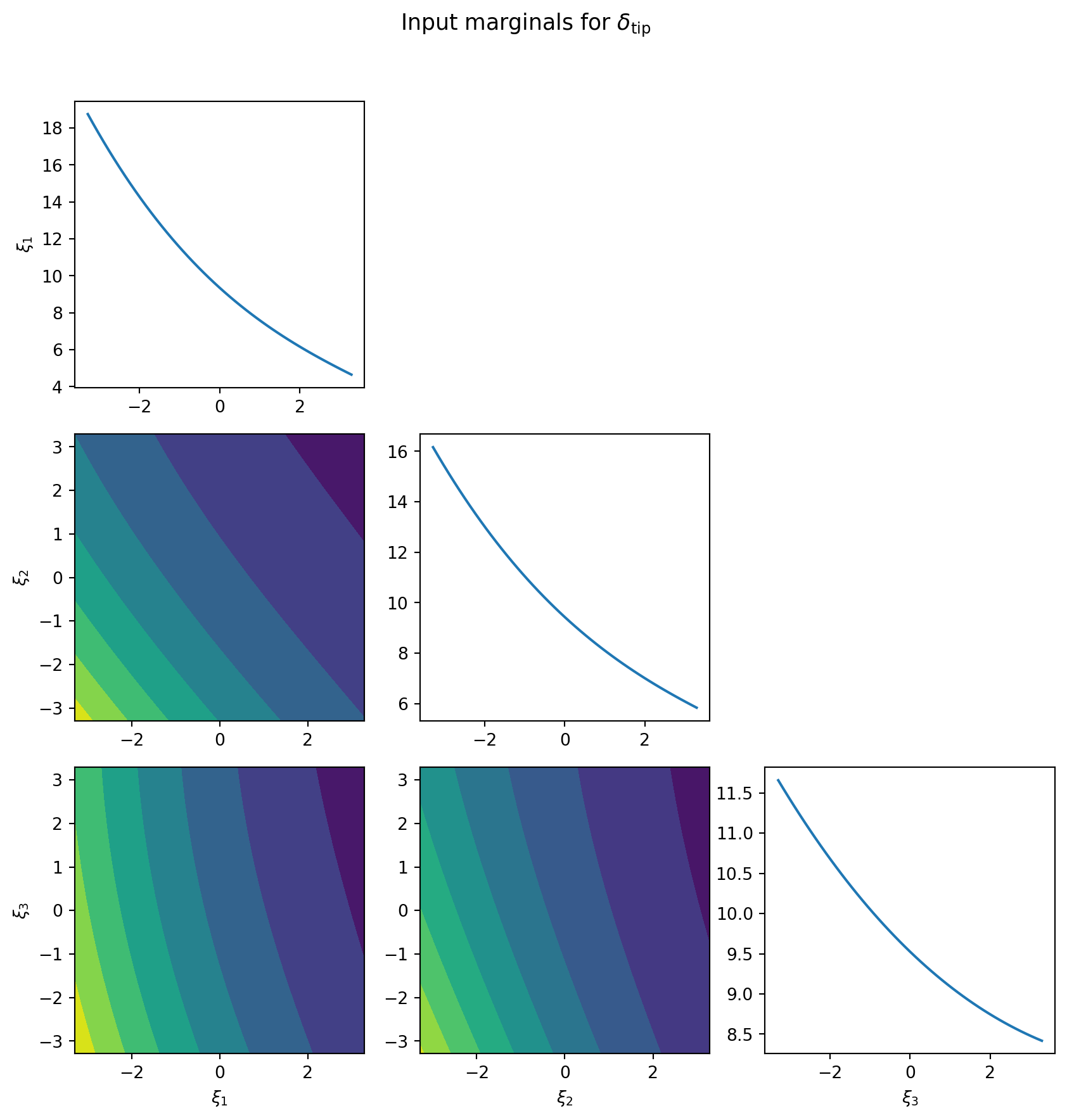
PCE vs. Monte Carlo: Efficiency Comparison
We now compare the efficiency of PCE-based moment estimation against direct Monte Carlo. The question is: for a fixed budget of \(N\) model evaluations, which approach gives more accurate estimates of the mean and variance?
For Monte Carlo, we use all \(N\) samples directly. For PCE, we increase the polynomial degree with the budget, keeping an oversampling ratio of 2 (twice as many samples as basis terms). This lets the PCE error decay as the budget grows, since higher-degree expansions capture more of the model’s structure.
Figure 3 repeats each experiment 20 times with different random seeds and plots the median error with 10th/90th percentile envelopes.
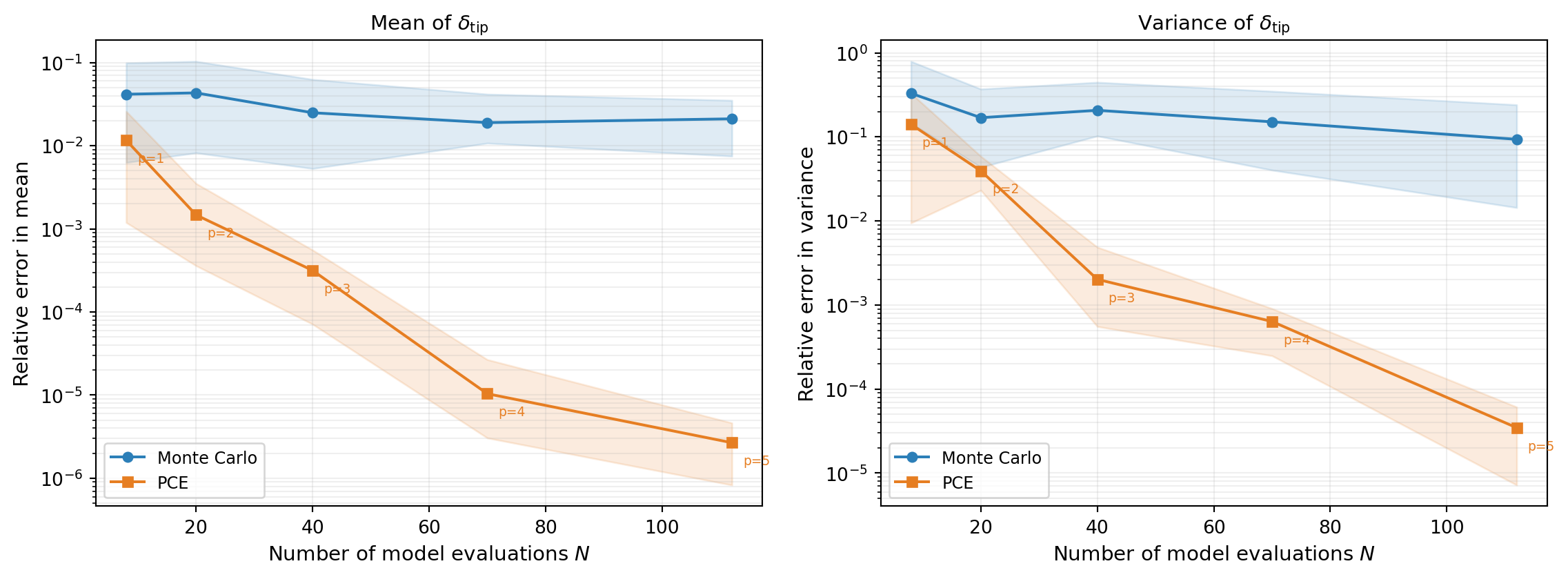
The PCE achieves lower error than Monte Carlo for the same computational budget because:
- Monte Carlo converges at rate \(1/\sqrt{N}\), regardless of the function’s smoothness.
- PCE converges at a rate determined by the smoothness of \(f\) — for smooth functions (like the beam model), polynomial convergence is much faster.
- By increasing the polynomial degree with the budget, the PCE error continues to decay, while MC progress is slow and steady.
Key Takeaways
- The orthonormality of the PCE basis gives analytical formulas for mean, variance, and covariance — no sampling required
- A cheap surrogate enables smooth density estimation from very large samples, which would be impractical with the expensive model
- Input marginalization is analytical for PCEs — only terms with degree 0 in the marginalized variables survive, giving exact main effect and interaction plots
- For smooth models, PCE-based moment estimation outperforms Monte Carlo at the same computational budget
Exercises
Compare the PCE-estimated correlation \(\text{Corr}[\delta_{\text{tip}}, \sigma_{\text{int}}]\) against a Monte Carlo estimate using 500 and 2000 model evaluations. How many MC samples are needed to match the PCE estimate?
Extract Sobol sensitivity indices via
pce.total_sobol_indices()andpce.main_effect_sobol_indices(). Which input variable contributes most to the variance of each QoI?In the convergence comparison (see Figure 3), change the oversampling ratio from 2 to 3. How does this affect the PCE error, especially at lower degrees?
Next Steps
- Overfitting and Cross-Validation — Choose the polynomial degree using LOO cross-validation
- Sparse Polynomial Approximation — OMP and BPDN/LASSO for high-dimensional polynomial chaos