
What Variational Inference Optimizes
PyApprox Tutorial Library
The KL divergence, the evidence problem, and the ELBO — the objective function behind VI.
TipDownload Notebook
Learning Objectives
After completing this tutorial, you will be able to:
- Interpret the KL divergence as a measure of mismatch between two distributions
- Explain why the KL divergence cannot be computed directly for posterior inference
- Derive the ELBO from the KL divergence using Bayes’ theorem
- Decompose the ELBO into its two competing terms and explain what each one does
- Visualize the ELBO landscape and identify how it balances data fit against prior regularization
Prerequisites
Complete Approximating the Posterior: Introduction to Variational Inference before this tutorial.
How Does VI Know Which Distribution Is Best?
The previous tutorial showed the optimizer improving a Gaussian fit to the posterior, but treated the objective as a black box. This tutorial opens the box. The central question: given two candidate Gaussians, how do we score which one is closer to the true posterior?
Measuring Mismatch Visually
Before writing any formulas, consider what “closeness” should mean. Figure 1 shows three candidate Gaussians overlaid on the exact beam posterior. The shaded regions highlight where each candidate disagrees with the posterior: the candidate places mass where the posterior is low, or misses mass where the posterior is high.
A good approximation places mass where the posterior has mass, and avoids placing mass where it does not. We need a single number that captures this.
The KL Divergence
The standard measure of mismatch in VI is the Kullback-Leibler (KL) divergence:
\[ \mathrm{KL}\!\big(q(\theta) \,\|\, p(\theta \mid y)\big) = \int q(\theta) \log \frac{q(\theta)}{p(\theta \mid y)} \, d\theta \]
Three properties make this a natural choice:
- It is always \(\geq 0\).
- It equals zero only when \(q\) and \(p\) match exactly.
- It penalizes \(q\) for placing mass where \(p(\theta \mid y)\) is small — exactly the pink-shaded mismatch in Figure 1.
To make this concrete, Figure 2 evaluates the KL divergence for every possible Gaussian \(q_{\mu, \sigma}\) on the 1D beam problem. The result is a surface over \((\mu, \sigma)\), and VI is searching for its minimum.
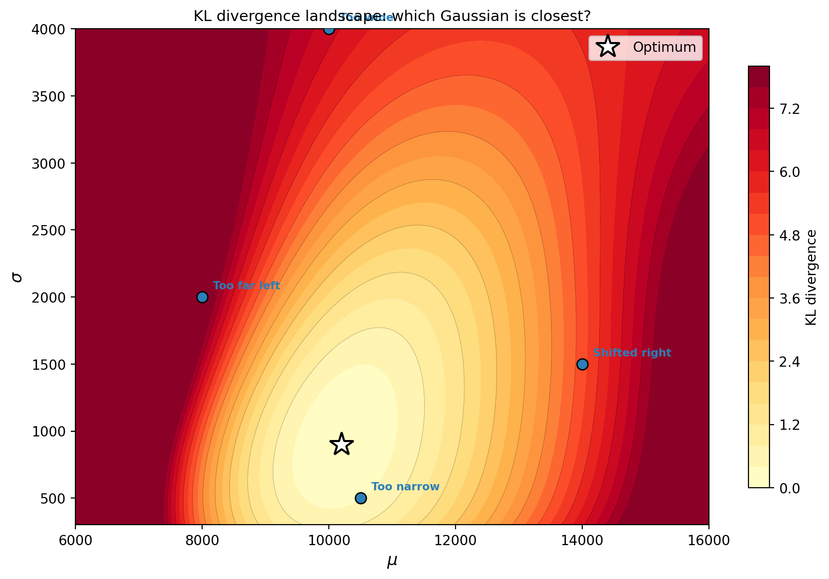
The poorly-fit candidates sit high on the KL surface. The optimal Gaussian sits at the bottom. VI’s optimizer descends this surface to find the minimum.
ImportantThe KL divergence is not symmetric
\(\mathrm{KL}(q \| p) \neq \mathrm{KL}(p \| q)\) in general. VI uses \(\mathrm{KL}(q \| p)\), which penalizes \(q\) for placing mass where \(p\) is small. This means VI with a unimodal \(q\) tends to concentrate on a single mode of the posterior rather than spreading across all modes — the “mode-seeking” behavior we saw in Tutorial 1’s bimodal example.
The Evidence Problem
There is an immediate obstacle to minimizing the KL divergence. The posterior \(p(\theta \mid y)\) in the formula involves the evidence (also called the marginal likelihood):
\[ p(\theta \mid y) = \frac{\mathcal{L}(\theta)\, p(\theta)}{p(y)}, \qquad p(y) = \int \mathcal{L}(\theta)\, p(\theta) \, d\theta \]
This integral is exactly the quantity that makes Bayesian inference hard in the first place. If we could compute \(p(y)\), we would already have the posterior and would not need VI. We need a way to optimize the KL divergence without computing \(p(y)\).
The ELBO
The solution is an algebraic trick. Substitute \(p(\theta \mid y) = \mathcal{L}(\theta) p(\theta) / p(y)\) into the KL divergence and rearrange:
\[ \mathrm{KL}(q \| p) = -\left[\mathbb{E}_{q}\!\big[\log \mathcal{L}(\theta)\big] - \mathrm{KL}\!\big(q(\theta) \,\|\, p(\theta)\big)\right] + \log p(y) \]
The evidence \(\log p(y)\) is a constant with respect to \(q\) — it does not depend on our choice of approximation. So minimizing the KL divergence is equivalent to maximizing the expression in brackets, which is called the Evidence Lower Bound (ELBO):
\[ \text{ELBO}(q) = \underbrace{\mathbb{E}_{q}\!\big[\log \mathcal{L}(\theta)\big]}_{\text{fit the data}} - \underbrace{\mathrm{KL}\!\big(q(\theta) \,\|\, p(\theta)\big)}_{\text{stay close to prior}} \tag{1}\]
Two Competing Terms
The ELBO has two terms that pull in opposite directions:
- The expected log-likelihood pushes \(q\) toward regions where the model predictions match the observations. On its own, this would collapse \(q\) onto the maximum likelihood estimate.
- The KL from prior penalizes \(q\) for straying from the prior. On its own, this would keep \(q\) equal to the prior regardless of the data.
The ELBO balances these forces — just as Bayes’ theorem balances the likelihood and the prior. Figure 3 shows each term separately, and their combination, as a function of the variational mean \(\mu\).
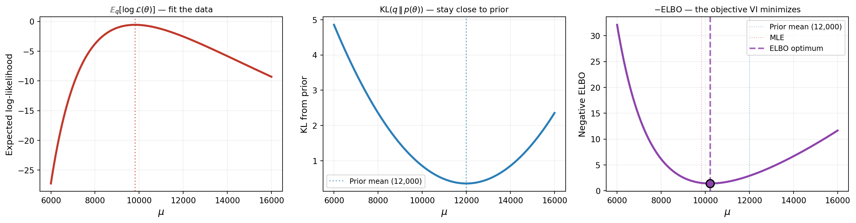
The ELBO optimum sits between the prior mean and the MLE — right where we expect the posterior to be. This is not a coincidence: the ELBO is a direct expression of the same prior-versus-data compromise that defines the posterior.
NoteWhy “Evidence Lower Bound”?
Since \(\mathrm{KL}(q \| p) \geq 0\), the rearrangement gives \(\text{ELBO}(q) \leq \log p(y)\) for any \(q\). The ELBO is a lower bound on the log-evidence, and the bound is tight when \(q\) equals the true posterior.
What We Defer
This tutorial derived the objective that VI optimizes. But we have not yet addressed how to compute gradients of the ELBO — the expected log-likelihood involves an integral over \(q\), which itself depends on the parameters we are tuning. The next tutorial introduces the reparameterization trick that makes this possible, and shows the optimization in action.
Key Takeaways
- The KL divergence measures how well \(q\) approximates the posterior: it penalizes \(q\) for placing mass where the posterior is low
- The KL divergence cannot be computed directly because it involves the intractable evidence \(p(y)\)
- The ELBO sidesteps this: maximizing the ELBO is equivalent to minimizing the KL divergence, and the ELBO only requires the likelihood and the prior
- The ELBO is a sum of two competing terms: fit the data (expected log-likelihood) and stay close to the prior (KL penalty)
- The ELBO’s minimum balances these forces in the same way that the posterior balances the likelihood and the prior
Exercises
In Figure 2, the KL surface appears to have a single minimum. Why must this be the case when the posterior is unimodal and the variational family is Gaussian? Hint: think about when \(\mathrm{KL}(q \| p) = 0\).
In Figure 3, increase the noise standard deviation to \(5 \times\) its current value (making the data less informative). How does the expected log-likelihood curve change? Does the ELBO optimum move closer to the prior mean or the MLE?
Decrease the prior standard deviation to \(500\) (a very informative prior). How does the KL-from-prior term change? What happens to the ELBO optimum when the prior is much more confident than the data?
(Challenge) For the special case where both the prior and the likelihood are Gaussian (so the true posterior is also Gaussian), derive the ELBO in closed form as a function of \((\mu, \sigma)\) using the known expression for the KL divergence between two Gaussians. Verify that the optimal \((\mu, \sigma)\) match the exact posterior parameters.
Next Steps
Continue with:
- Optimizing the ELBO — The reparameterization trick, convergence monitoring, and practical VI