---
title: "PACV: Analysis"
subtitle: "PyApprox Tutorial Library"
description: "Formal definition of the three PACV estimator families (GMF, GRD, GIS), how the recursion index determines allocation matrix structure, and the covariance formulas that enable enumeration-based best-estimator selection."
tutorial_type: analysis
topic: multi_fidelity
difficulty: advanced
estimated_time: 20
render_time: 77
prerequisites:
- pacv_concept
- acv_many_models_analysis
tags:
- multi-fidelity
- pacv
- gmf
- grd
- gis
- allocation-matrix
- estimator-theory
format:
html:
code-fold: false
code-tools: true
toc: true
execute:
echo: true
warning: false
jupyter: python3
---
::: {.callout-tip collapse="true"}
## Download Notebook
[Download as Jupyter Notebook](notebooks/pacv_analysis.ipynb)
:::
## Learning Objectives
After completing this tutorial, you will be able to:
- Write the allocation matrix for any GMF, GRD, or GIS estimator given its recursion
index $\boldsymbol{\gamma}$
- Identify which cells of the allocation matrix change when $\boldsymbol{\gamma}$ changes
- State the partition size formula and how it translates a budget into sample counts for
each partition
- Verify that MLMC, MFMC, ACVMF, and ACVIS are recovered as special cases
- Describe the enumeration procedure that PyApprox uses to select the best estimator
## Prerequisites
Complete [PACV Concept](pacv_concept.qmd) and
[General ACV Analysis](acv_many_models_analysis.qmd) before this tutorial.
The [ACV Allocation Matrices](acv_many_models_analysis.qmd#sec-allocation-matrix) reference provides supporting
detail on the notation used throughout.
## Notation
We follow the notation from [General ACV Analysis](acv_many_models_analysis.qmd).
Models are $f_0$ (HF) through $f_M$ (cheapest LF). The recursion index is
$\boldsymbol{\gamma} = [\gamma_1, \ldots, \gamma_M]^\top$ with $0 \leq \gamma_j < j$.
Recall from [ACV Allocation Matrices](acv_many_models_analysis.qmd#sec-allocation-matrix): the allocation
matrix $\mathbf{A} \in \{0,1\}^{(M+1)\times 2(M+1)}$ has entry $A_{ij} = 1$ if
partition $\mathcal{P}_i$ is included in $\mathcal{Z}_\alpha^*$ (column $2\alpha-1$)
or $\mathcal{Z}_\alpha$ (column $2\alpha$). The first column is always zero ($\mathcal{Z}_0^*$
is not used).
## The GMF Family
**Generalised Multi-Fidelity (GMF)** estimators use a base allocation matrix derived from
the MFMC structure. For a given recursion index $\boldsymbol{\gamma}$, the rule is:
> If $\gamma_j = i$, then $\mathcal{Z}_j^* = \mathcal{Z}_i$
> **and** $\mathcal{Z}_i \subseteq \mathcal{Z}_j$.
The second condition — the anchor is a *nested subset* — is the MFMC inheritance.
Translating to the allocation matrix: partition $\mathcal{P}_k$ is included in
$\mathcal{Z}_j$ if $\mathcal{P}_k \subseteq \mathcal{Z}_{\gamma_j} \subseteq \mathcal{Z}_j$.
**Special cases:**
- $\boldsymbol{\gamma} = [0, 1, \ldots, M-1]$ (chain) $\Rightarrow$ MFMC
- $\boldsymbol{\gamma} = [0, 0, \ldots, 0]$ (star) $\Rightarrow$ ACVMF
For the three-model ($M=2$) case, the two GMF allocation matrices are:
$$
\boldsymbol{\gamma} = [0, 1]: \quad
\mathbf{A}_{\text{GMF}} =
\begin{pmatrix}
0 & 1 & 1 & 1 & 1 & 1 \\
0 & 0 & 0 & 1 & 1 & 1 \\
0 & 0 & 0 & 0 & 0 & 1
\end{pmatrix}
= \mathbf{A}_\text{MFMC}
$$
$$
\boldsymbol{\gamma} = [0, 0]: \quad
\mathbf{A}_{\text{GMF}} =
\begin{pmatrix}
0 & 1 & 1 & 1 & 1 & 1 \\
0 & 0 & 0 & 1 & 0 & 1 \\
0 & 0 & 0 & 0 & 0 & 1
\end{pmatrix}
= \mathbf{A}_\text{ACVMF}
$$
The difference is in row 1, column 4 (model $f_1$'s $\mathcal{Z}_2^*$ column): in MFMC
($\gamma_2=1$), $f_1$'s sample set is the anchor for $f_2$, so partition $\mathcal{P}_1$
is included in $\mathcal{Z}_2^*$. In ACVMF ($\gamma_2=0$), $f_0$'s set is the anchor,
so $\mathcal{P}_1 \not\subseteq \mathcal{Z}_2^*$.
```{python}
import numpy as np
import matplotlib.pyplot as plt
from pyapprox.util.backends.numpy import NumpyBkd
from pyapprox_benchmarks.statest import (
    PolynomialEnsembleBenchmark,
)
from pyapprox.statest.statistics import MultiOutputMean
from pyapprox.statest.mc_estimator import MCEstimator
from pyapprox.statest.acv import GMFEstimator, GRDEstimator, GISEstimator
from pyapprox.statest.acv.search import ACVSearch
from pyapprox.statest.acv.allocation import ACVAllocator, default_allocator_factory
from pyapprox.statest.acv.base import FittedACVEstimator
from pyapprox.statest.acv.strategies import (
    FixedRecursionStrategy, TreeDepthRecursionStrategy,
)
from pyapprox.statest.allocation import MCAllocator
from pyapprox.statest.plotting import plot_allocation
from pyapprox.optimization.minimize.scipy.slsqp import ScipySLSQPOptimizer

bkd = NumpyBkd()
np.random.seed(1)
benchmark = PolynomialEnsembleBenchmark(bkd, nmodels=5)
nmodels   = 4
costs     = benchmark.problem().costs()[:nmodels]
cov       = benchmark.ensemble_covariance()[:nmodels, :nmodels]
nqoi      = benchmark.problem().models()[0].nqoi()

stat = MultiOutputMean(nqoi, bkd)
stat.set_pilot_quantities(cov)

# Use SLSQP-only allocator for fast search (no DE global search needed for
# this small problem with M=3 LF models)
_slsqp = ScipySLSQPOptimizer(maxiter=200)
def fast_allocator(est):
    """Route analytical cases to closed-form, others to SLSQP."""
    alloc = default_allocator_factory(est)
    if isinstance(alloc, ACVAllocator):
        return ACVAllocator(est, optimizer=_slsqp)
    return alloc

# MFMC (chain) and ACVMF (star) as GMF estimators
ri_chain = (0, 1, 2)   # M=3 LF models
ri_star  = (0, 0, 0)

fig, axes = plt.subplots(1, 2, figsize=(14, 5))
for ax, ri, title in zip(
    axes,
    [ri_chain, ri_star],
    [r"GMF with $\boldsymbol{\gamma}=[0,1,2]$ (= MFMC)",
     r"GMF with $\boldsymbol{\gamma}=[0,0,0]$ (= ACVMF)"],
):
    search = ACVSearch(stat, costs, recursion_strategy=FixedRecursionStrategy(ri),
                       allocator_factory=fast_allocator)
    try:
        result = search.search(500.0)
        plot_allocation(result.best, ax, show_partition_sizes=True)
    except RuntimeError:
        ax.text(0.5, 0.5, "opt. failed", ha="center", va="center",
                fontsize=9, transform=ax.transAxes)
    ax.set_title(title, fontsize=10)
plt.suptitle("GMF allocation matrices: chain vs star recursion index", fontsize=11)
plt.tight_layout()
plt.show()
```
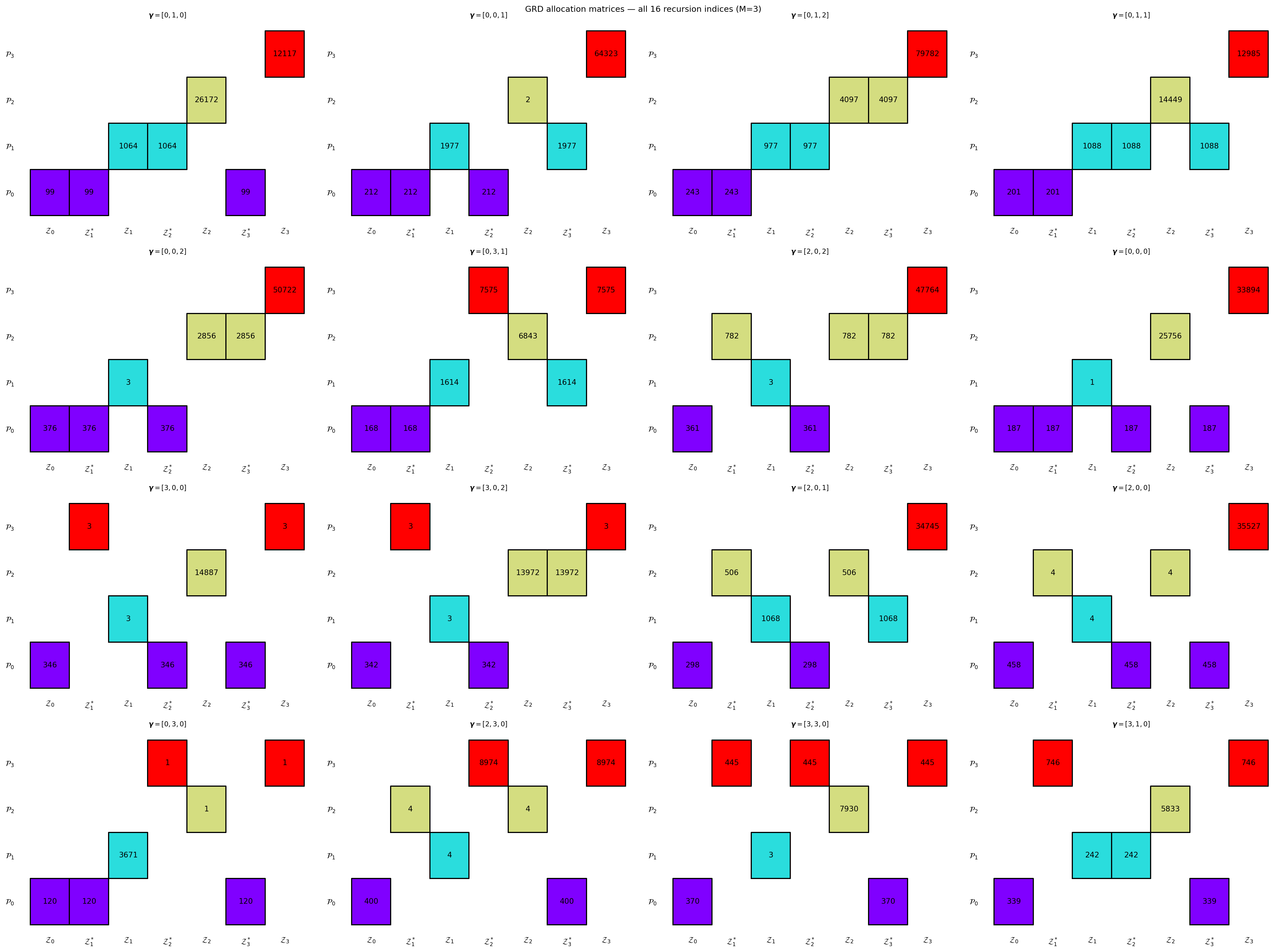
## The GRD Family
**Generalised Recursive Difference (GRD)** estimators use the MLMC allocation matrix
as base. The rule is:
> If $\gamma_j = i$, then $\mathcal{Z}_j^* = \mathcal{Z}_i$
> **and** if $i \neq j$, then $\mathcal{Z}_i \cap \mathcal{Z}_j \neq \emptyset$
> (overlapping but neither nested in the other).
This gives the recursive-difference structure of MLMC at every edge in the DAG.
**Special case:** $\boldsymbol{\gamma} = [0, 1, \ldots, M-1]$ (chain) $\Rightarrow$ MLMC.
```{python}
#| fig-cap: "GRD allocation matrices for all valid recursion indices with $M=3$ LF models, showing how the partition structure changes as edges in the DAG are rewired."
#| label: fig-grd-matrices
search_grd = ACVSearch(
    stat, costs,
    estimator_classes=[GRDEstimator],
    recursion_strategy=TreeDepthRecursionStrategy(max_depth=nmodels - 1),
    allocator_factory=fast_allocator,
)
result_grd = search_grd.search(500.0, allow_failures=True)

n     = len(result_grd.all_allocations)
ncols = min(n, 4)
nrows = (n + ncols - 1) // ncols
fig, axes = plt.subplots(nrows, ncols, figsize=(ncols * 6, nrows * 4.5))
axes = np.array(axes).ravel()

for i, (est, alloc) in enumerate(result_grd.all_allocations):
    ri = bkd.to_numpy(est._recursion_index).astype(int).tolist()
    if alloc.success:
        fitted = FittedACVEstimator(est, alloc)
        plot_allocation(fitted, axes[i], show_partition_sizes=True)
    else:
        axes[i].text(0.5, 0.5, "opt. failed", ha="center", va="center",
                     fontsize=9, transform=axes[i].transAxes)
    axes[i].set_title(rf"$\boldsymbol{{\gamma}}={list(ri)}$", fontsize=9)

for ax in axes[n:]:
    ax.set_visible(False)

plt.suptitle(f"GRD allocation matrices — all {n} recursion indices (M={nmodels-1})", fontsize=11)
plt.tight_layout()
plt.show()
```
## The GIS Family
**Generalised Independent Sample (GIS)** estimators use the ACVIS allocation matrix
as base. The rule is:
> If $\gamma_j = i$, then $\mathcal{Z}_j^* \subseteq \mathcal{Z}_j$
> and $\mathcal{Z}_j^*$ is the same *independent* sub-partition as $\mathcal{Z}_i$'s anchor.
The key distinction from GMF and GRD: the anchor and the full set of $f_j$ are drawn
from **independent partitions**, giving uncorrelated corrections across different models.
This is the generalisation of ACVIS's independent sample structure.
**Special case:** $\boldsymbol{\gamma} = [0, 0, \ldots, 0]$ (star) $\Rightarrow$ ACVIS.
```{python}
#| fig-cap: "GIS allocation matrices for all valid recursion indices with $M=3$ LF models."
#| label: fig-gis-matrices
search_gis = ACVSearch(
    stat, costs,
    estimator_classes=[GISEstimator],
    recursion_strategy=TreeDepthRecursionStrategy(max_depth=nmodels - 1),
    allocator_factory=fast_allocator,
)
result_gis = search_gis.search(500.0, allow_failures=True)

fig, axes = plt.subplots(nrows, ncols, figsize=(ncols * 6, nrows * 4.5))
axes = np.array(axes).ravel()

for i, (est, alloc) in enumerate(result_gis.all_allocations):
    ri = bkd.to_numpy(est._recursion_index).astype(int).tolist()
    if alloc.success:
        fitted = FittedACVEstimator(est, alloc)
        plot_allocation(fitted, axes[i], show_partition_sizes=True)
    else:
        axes[i].text(0.5, 0.5, "opt. failed", ha="center", va="center",
                     fontsize=9, transform=axes[i].transAxes)
    axes[i].set_title(rf"$\boldsymbol{{\gamma}}={list(ri)}$", fontsize=9)

for ax in axes[n:]:
    ax.set_visible(False)

plt.suptitle(f"GIS allocation matrices — all {n} recursion indices (M={nmodels-1})", fontsize=11)
plt.tight_layout()
plt.show()
```
## Partition Sizes and the Budget Constraint
For any PACV estimator with allocation matrix $\mathbf{A}$, the cost of a sample in
partition $\mathcal{P}_k$ is the sum of costs of all models that evaluate it:
$$
c_k = \sum_{\alpha=0}^{M} C_\alpha \cdot \mathbf{1}[\mathcal{P}_k \subseteq \mathcal{Z}_\alpha].
$$
The budget constraint is $\sum_k p_k c_k \leq P$. The optimal partition sizes
$\mathbf{p}^*$ are found by solving
$$
\min_{\mathbf{p} \geq 0} \;\det\!\left[\boldsymbol{\Sigma}_{Q_0 Q_0}
- \boldsymbol{\Sigma}_{Q_0\Delta}(\mathbf{p})\,
\boldsymbol{\Sigma}_{\Delta\Delta}(\mathbf{p})^{-1}\,
\boldsymbol{\Sigma}_{\Delta Q_0}(\mathbf{p})\right]
\quad\text{s.t.}\quad \sum_k p_k c_k \leq P.
$$ {#eq-alloc-opt}
PyApprox solves this via `ACVSearch.search(P)` using a quasi-Newton (SLSQP) optimiser.
For a fixed allocation matrix, the objective is smooth in $\mathbf{p}$ and the
optimisation typically converges in tens of iterations.
::: {.callout-note}
## Why not solve over all recursion indices simultaneously?
Optimising $\mathbf{p}$ and $\boldsymbol{\gamma}$ jointly would require mixed-integer
programming. PACV sidesteps this by decoupling: enumerate all $M!$ indices, solve the
continuous optimisation @eq-alloc-opt for each, then pick the best. This is exact and
inexpensive for typical ensemble sizes.
:::
## How `get_all_recursion_indices` Works
The valid recursion indices form a product space:
$\gamma_j \in \{0, \ldots, j-1\}$ for $j = 1, \ldots, M$.
The total count is $\prod_{j=1}^M j = M!$.
```{python}
print("Recursion index counts by M:")
import math
for M in range(1, 7):
    n_ri = math.factorial(M)
    print(f"  M={M} LF models: {n_ri:5d} valid recursion indices")

# Verify against PyApprox
rec_strat = TreeDepthRecursionStrategy(max_depth=nmodels - 1)
all_ri    = rec_strat.indices(nmodels, bkd)
print(f"\nPyApprox returned {len(all_ri)} indices for M={nmodels-1}: {[bkd.to_numpy(ri).astype(int).tolist() for ri in all_ri[:6]]}...")
```
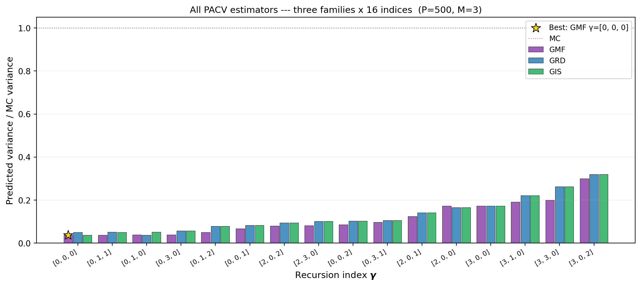
## Cross-Family Variance Comparison
For any fixed recursion index, the three families produce different allocation matrices
and hence different variance reductions. @fig-cross-family compares GMF, GRD, and GIS
for every valid recursion index at a fixed budget.
```{python}
#| fig-cap: "Predicted variance (relative to MC) for every valid recursion index across all three PACV families on the four-model polynomial benchmark at $P = 500$. The best overall estimator is highlighted. Families differ by their base allocation structure; the recursion index shifts the optimum within each family."
#| label: fig-cross-family
fam_cols    = {"gmf": "#8E44AD", "grd": "#2C7FB8", "gis": "#27AE60"}
fam_names   = {"gmf": "GMF", "grd": "GRD", "gis": "GIS"}

mc_est = MCEstimator(stat, costs[:1])
mc_fitted = MCAllocator(mc_est).allocate(500.0)
mc_var = float(bkd.to_numpy(mc_fitted.covariance())[0, 0])

# GMF search (GRD and GIS reuse result_grd, result_gis from above)
search_gmf = ACVSearch(
    stat, costs,
    estimator_classes=[GMFEstimator],
    recursion_strategy=TreeDepthRecursionStrategy(max_depth=nmodels - 1),
    allocator_factory=fast_allocator,
)
result_gmf = search_gmf.search(500.0, allow_failures=True)

# Extract per-index variances from each family's cached results
results = {}
ri_list = None
for fam, result_fam in [("gmf", result_gmf), ("grd", result_grd), ("gis", result_gis)]:
    fam_vars = []
    fam_ri = []
    for est, alloc in result_fam.all_allocations:
        ri = bkd.to_numpy(est._recursion_index).astype(int).tolist()
        fam_ri.append(ri)
        if alloc.success:
            fitted = FittedACVEstimator(est, alloc)
            var = float(bkd.to_numpy(fitted.covariance())[0, 0])
        else:
            var = mc_var
        fam_vars.append(var / mc_var)
    results[fam] = fam_vars
    if ri_list is None:
        ri_list = fam_ri

from pyapprox_tutorials.figures._multifidelity_advanced import plot_pacv_cross_family

fig, ax = plt.subplots(figsize=(11, 5))
plot_pacv_cross_family(ri_list, results, fam_names, fam_cols, mc_var,
                       nmodels, ax)
plt.tight_layout()
plt.show()
```
## Relationship to the General ACV Formula
Every PACV estimator fits the general ACV framework from
[General ACV Analysis](acv_many_models_analysis.qmd). For a given recursion index and
family, the allocation matrix determines the sample-set intersection sizes, which
in turn determine $\boldsymbol{\Sigma}_{\Delta\Delta}$ and $\boldsymbol{\Sigma}_{\Delta Q_0}$.
The optimal variance formula is always the Schur-complement form from that tutorial:
$$
\mathbb{C}\mathrm{ov}(\hat{\mathbf{Q}}_0^{\text{ACV}})
= \boldsymbol{\Sigma}_{Q_0 Q_0}
- \boldsymbol{\Sigma}_{Q_0\Delta}\,\boldsymbol{\Sigma}_{\Delta\Delta}^{-1}\,
\boldsymbol{\Sigma}_{\Delta Q_0}.
$$
What PACV adds is a systematic way to parametrise and search the space of all allocation
matrices, rather than considering only the four classical designs.
## Key Takeaways
- **GMF** uses nested anchor sets ($\mathcal{Z}_i \subseteq \mathcal{Z}_j$); contains
MFMC and ACVMF as special cases
- **GRD** uses overlapping (but not nested) anchor sets; contains MLMC as a special case
- **GIS** uses independent anchor sub-partitions; contains ACVIS as a special case
- The allocation matrix is fully determined by the recursion index + family; the
covariance formula $\boldsymbol{\Sigma}_{\Delta\Delta}(\mathbf{p})$ is then tractable
- The enumeration procedure is: generate all $M!$ recursion indices, solve
@eq-alloc-opt for each, pick the minimum variance — no additional model evaluations
beyond the pilot
## Exercises
1. Write the GMF allocation matrix for $M=2$ with $\boldsymbol{\gamma}=[0,1]$
(MFMC) and $\boldsymbol{\gamma}=[0,0]$ (ACVMF) explicitly. Confirm they match
the matrices given in the text.
2. For the GRD family with $\boldsymbol{\gamma}=[0,0,0]$: what does the allocation
matrix look like? What classical estimator (if any) does this correspond to?
3. From @fig-cross-family, does the best recursion index for GMF match the best for GRD
and GIS? What does this suggest about whether family choice matters independently of
recursion index?
4. **(Challenge)** Show that for a two-model problem ($M=1$), all three families produce
the same allocation matrix for $\boldsymbol{\gamma}=[0]$. Why does the distinction
between families only arise for $M \geq 2$?
## References
- [BLWLJCP2022] G.F. Bomarito, P.E. Leser, J.E. Warner, W.P. Leser. *On the optimization
of approximate control variates with parametrically defined estimators.* Journal of
Computational Physics, 451:110882, 2022.
[DOI](https://doi.org/10.1016/j.jcp.2021.110882)
- [GGEJJCP2020] A. Gorodetsky, S. Geraci, M. Eldred, J. Jakeman. *A generalized
approximate control variate framework for multifidelity uncertainty quantification.*
Journal of Computational Physics, 408:109257, 2020.
[DOI](https://doi.org/10.1016/j.jcp.2020.109257)