Leja Sequences: Nested Points for Adaptive Interpolation

PyApprox Tutorial Library

Construct Leja sequences via greedy determinant maximization, understand Christoffel weighting, compare one-point vs. two-point optimization, and compare Leja vs. Gauss vs. CC for interpolation accuracy.

TipDownload Notebook

Download as Jupyter Notebook

Learning Objectives

After completing this tutorial, you will be able to:

• Explain why nestedness matters for adaptive algorithms and sparse grids
• Define Leja points via greedy weighted determinant maximization
• Understand the role of the Christoffel function as a weighting
• Construct Leja sequences using LejaSequence1D with ChristoffelWeighting
• Compare one-point vs. two-point optimized Leja sequences for improved quadrature accuracy
• Compare Leja vs. Gauss vs. Clenshaw-Curtis interpolation convergence
• Build probability-aware Leja sequences for non-uniform distributions

Prerequisites

Complete Lagrange Interpolation before this tutorial. You should understand Lagrange basis polynomials and why point placement affects convergence.

Setup

import numpy as np
np.random.seed(42)
import matplotlib.pyplot as plt

from pyapprox.util.backends.numpy import NumpyBkd

from pyapprox.surrogates.affine.univariate import (
    JacobiPolynomial1D,
    LegendrePolynomial1D,
    GaussQuadratureRule,
    LagrangeBasis1D,
)
from pyapprox.surrogates.affine.univariate.globalpoly import (
    ClenshawCurtisQuadratureRule,
)
from pyapprox.surrogates.affine.leja import (
    LejaSequence1D,
    ChristoffelWeighting,
)
from pyapprox.surrogates.sparsegrids import LejaLagrangeFactory

bkd = NumpyBkd()

Why Nestedness Matters

Both Gauss-Legendre and Clenshaw-Curtis rules produce accurate quadrature, but they are designed to be used at a fixed number of points \(M\). When we want to increase accuracy by adding more points, neither rule naturally reuses existing evaluations: a Gauss-\(M\) grid and a Gauss-\((M+2)\) grid share no points.

For adaptive algorithms that refine iteratively — and for sparse grids (Tutorial 6) that build approximations by combining sub-grids at different levels — nested point sets are essential. A family of point sets \(\mathcal{Z}_1 \subset \mathcal{Z}_2 \subset \mathcal{Z}_3 \subset \cdots\) is nested if every set at level \(\ell\) contains all points from level \(\ell - 1\). This means function evaluations from coarser levels are never wasted when the grid is refined.

Clenshaw-Curtis nodes are nested for the specific sequence \(M = 2^k + 1\), but this restricts how we can grow the grid. Leja sequences are a flexible alternative: they are nested by construction, they grow one point at a time, and they can be adapted to any probability measure.

Leja Points: Greedy Determinant Maximization

Given an existing set of \(M\) points \(\mathcal{Z}_M = \{z^{(1)}, \ldots, z^{(M)}\}\) on \([a, b]\), the next Leja point is chosen to maximize the product of distances to all existing points, weighted by a function \(v(z)\):

\[ z^{(M+1)} = \underset{z \in [a, b]}{\operatorname{argmax}}\; v(z) \prod_{n=1}^{M} \left\lvert z - z^{(n)} \right\rvert. \]

This is equivalent to maximizing the determinant of the Vandermonde matrix of the extended point set, and it ensures the new point is as far as possible (in a weighted sense) from all existing nodes — preventing clustering and controlling the Lebesgue constant.

The first point \(z^{(1)}\) is typically chosen as the maximum of \(v\) alone; subsequent points are selected greedily.

Figure 1: Leja sequence growth: the sequence at 3, 5, 9, and 15 points. Each new point fills the largest gap in the current set.

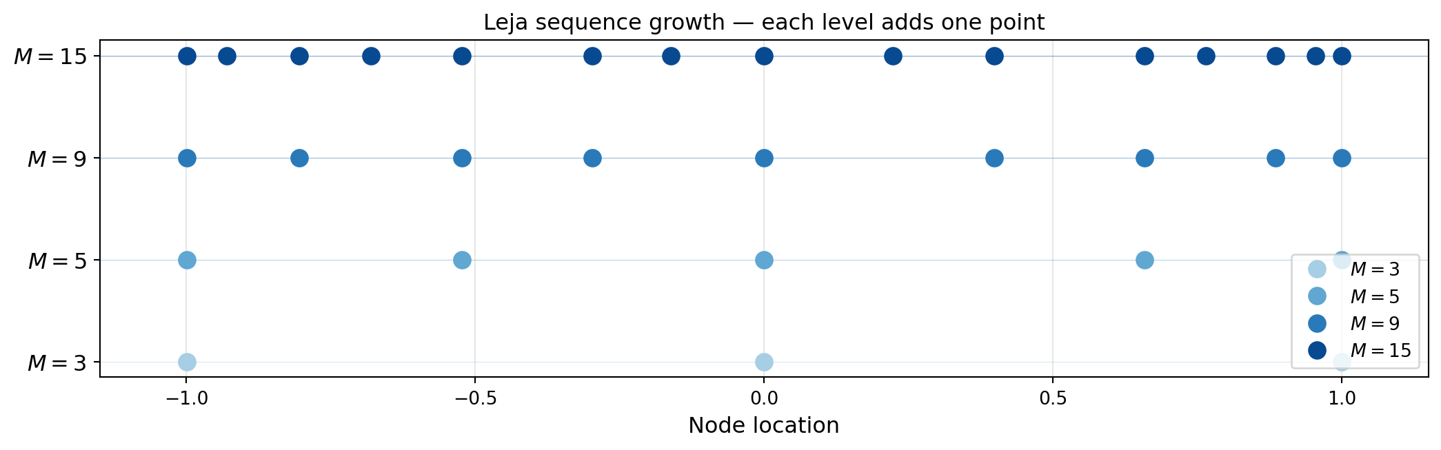
The key observation is that the 3-point sequence is a subset of the 15-point sequence. Any function values already computed at the 3-point level are reused exactly when the sequence grows to 15 points.

LejaSequence1D and ChristoffelWeighting

LejaSequence1D implements the greedy Leja construction for any distribution. It takes:

• A basis (orthogonal polynomial, e.g. JacobiPolynomial1D for uniform, LegendrePolynomial1D)
• A weighting (e.g. ChristoffelWeighting which uses the Christoffel function \(v(z) = \sqrt{K_M(z, z)}\), where \(K_M\) is the reproducing kernel)
• Bounds for the domain

The Christoffel function weighting makes the resulting points near-optimal for polynomial interpolation with respect to the target probability measure.

from pyapprox.tutorial_figures._interpolation import plot_node_distribution

# Build a Leja sequence on [-1, 1] with Christoffel weighting
poly_leg = LegendrePolynomial1D(bkd)
poly_leg.set_nterms(30)
weighting = ChristoffelWeighting(bkd)
leja = LejaSequence1D(bkd, poly_leg, weighting, bounds=(-1.0, 1.0))

# Get 15 Leja points
M = 15
nodes_leja, weights_leja = leja.quadrature_rule(M)

# Compare node distributions
cc_rule = ClenshawCurtisQuadratureRule(bkd, store=True)
nodes_cc, _ = cc_rule(17)   # 17 CC points (nearest valid CC size >= 15)

gauss_rule = GaussQuadratureRule(poly_leg, store=True)
nodes_gauss, _ = gauss_rule(M)

leja_np  = bkd.to_numpy(nodes_leja).ravel()
cc_np    = bkd.to_numpy(nodes_cc).ravel()
gauss_np = bkd.to_numpy(nodes_gauss).ravel()

fig, axs = plt.subplots(3, 1, figsize=(11, 5), sharex=True)
plot_node_distribution(leja_np, M, cc_np, 17, gauss_np, M, axs)
plt.suptitle("Node distributions — all cluster toward boundary", fontsize=12)
plt.tight_layout()
plt.show()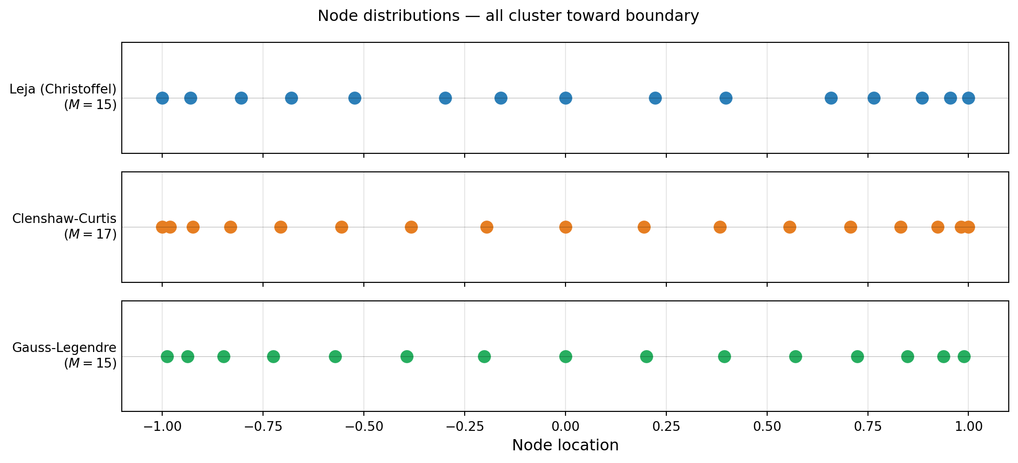

Nestedness verification

Leja sequences are nested by construction: the first \(M\) points of an \(N\)-point sequence (\(N > M\)) are identical to the \(M\)-point sequence.

# Verify nestedness
nodes5, _ = leja.quadrature_rule(5)
nodes10, _ = leja.quadrature_rule(10)
nodes15, _ = leja.quadrature_rule(15)

n5  = bkd.to_numpy(nodes5).ravel()
n10 = bkd.to_numpy(nodes10).ravel()
n15 = bkd.to_numpy(nodes15).ravel()

assert np.allclose(n5, n10[:5]), "5-pt not nested in 10-pt"
assert np.allclose(n10, n15[:10]), "10-pt not nested in 15-pt"

Using LagrangeBasis1D with Leja Points

LagrangeBasis1D accepts any quadrature rule callable with signature (npoints) → (samples, weights). We can pass leja.quadrature_rule directly:

from pyapprox.tutorial_figures._interpolation import plot_lagrange_on_leja

# Build a Lagrange basis on Leja points
basis_leja = LagrangeBasis1D(bkd, leja.quadrature_rule)
basis_leja.set_nterms(7)

# Evaluate at a fine grid
x_eval = bkd.array(np.linspace(-1, 1, 300).reshape(1, -1))
phi_leja = bkd.to_numpy(basis_leja(x_eval))     # (300, 7)
nodes_7, _ = basis_leja.quadrature_rule()
nodes_7_np = bkd.to_numpy(nodes_7).ravel()

x_plot = np.linspace(-1, 1, 300)

fig, ax = plt.subplots(figsize=(9, 4))
plot_lagrange_on_leja(x_plot, phi_leja, nodes_7_np, 7, ax)
plt.tight_layout()
plt.show()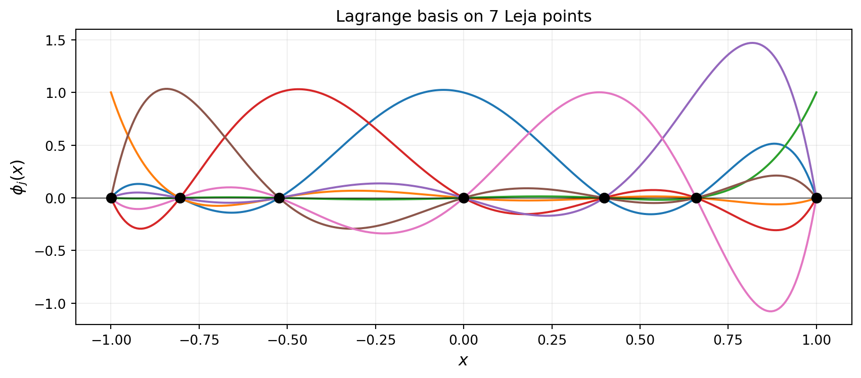

LejaLagrangeFactory for Sparse Grids

In the sparse grid framework (Tutorial 6), each dimension of the grid needs a factory object that produces the 1D basis at any requested level. LejaLagrangeFactory wraps the Leja sequence construction into this interface.

# LejaLagrangeFactory takes a marginal and backend;
# it lazily constructs a LejaSequence1D and wraps it
# as a LagrangeBasis1D.

from pyapprox.probability.univariate.uniform import UniformMarginal

marginal = UniformMarginal(-1.0, 1.0, bkd)
factory = LejaLagrangeFactory(marginal, bkd)

# The factory creates a LagrangeBasis1D backed by a Leja sequence
basis_from_factory = factory.create_basis()
basis_from_factory.set_nterms(5)
nodes_fac, weights_fac = basis_from_factory.quadrature_rule()

Convergence Comparison

For a uniform distribution the three families — Leja, Clenshaw-Curtis, and Gauss — all achieve exponential convergence for analytic functions. Leja sequences typically match CC accuracy for moderate \(M\) while retaining the flexibility to be grown one point at a time.

from pyapprox.tutorial_figures._interpolation import plot_leja_convergence

def f_test(x):
    return np.exp(np.cos(np.pi * x))


x_ref = np.linspace(-1.0, 1.0, 2000)
x_ref_bkd = bkd.array(x_ref.reshape(1, -1))
true_ref = f_test(x_ref)

# Build bases for each method
basis_leja_conv = LagrangeBasis1D(bkd, leja.quadrature_rule)
basis_gauss_conv = LagrangeBasis1D(bkd, gauss_rule)

Ms = list(range(3, 23))
err_leja, err_gauss = [], []

# CC only works for M = 1, 3, 5, 9, 17 — collect valid sizes
cc_Ms = [3, 5, 9, 17]
err_cc = []

for M in Ms:
    # Leja
    basis_leja_conv.set_nterms(M)
    nd_l, _ = basis_leja_conv.quadrature_rule()
    nd_l_np = bkd.to_numpy(nd_l).ravel()
    phi_l = bkd.to_numpy(basis_leja_conv(x_ref_bkd))
    interp_l = phi_l @ f_test(nd_l_np)
    err_leja.append(np.max(np.abs(true_ref - interp_l)))

    # Gauss
    basis_gauss_conv.set_nterms(M)
    nd_g, _ = basis_gauss_conv.quadrature_rule()
    nd_g_np = bkd.to_numpy(nd_g).ravel()
    phi_g = bkd.to_numpy(basis_gauss_conv(x_ref_bkd))
    interp_g = phi_g @ f_test(nd_g_np)
    err_gauss.append(np.max(np.abs(true_ref - interp_g)))

for M in cc_Ms:
    basis_cc_conv = LagrangeBasis1D(bkd, cc_rule)
    basis_cc_conv.set_nterms(M)
    nd_c, _ = basis_cc_conv.quadrature_rule()
    nd_c_np = bkd.to_numpy(nd_c).ravel()
    phi_c = bkd.to_numpy(basis_cc_conv(x_ref_bkd))
    interp_c = phi_c @ f_test(nd_c_np)
    err_cc.append(np.max(np.abs(true_ref - interp_c)))

fig, ax = plt.subplots(figsize=(9, 5))
plot_leja_convergence(Ms, err_leja, cc_Ms, err_cc, err_gauss, ax)
plt.tight_layout()
plt.show()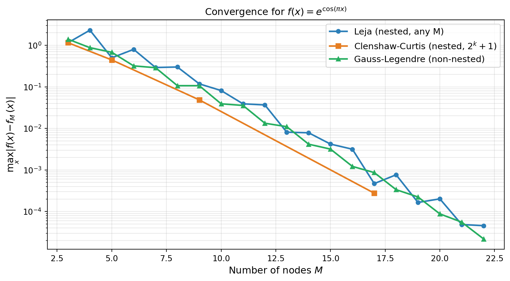

Figure 2: Interpolation error vs. M for an analytic function. Leja and CC achieve comparable exponential convergence; Gauss is slightly more efficient but non-nested.

All three methods converge exponentially for this analytic function. The advantage of Leja over Gauss is not accuracy per se, but flexibility: Leja sequences can be extended by a single point without discarding any existing evaluations.

Two-Point Optimized Leja Sequences

The standard Leja algorithm adds one point at a time, choosing it to maximize a one-dimensional objective. A natural improvement is to optimize two points simultaneously: given a sequence of \(M\) points, find the pair \((z^{(M+1)}, z^{(M+2)})\) that jointly maximizes the determinant of the extended Vandermonde-like matrix.

The TwoPointLejaObjective solves a 2D optimization problem at each step, maximizing the squared determinant of a \(2 \times 2\) weighted residual matrix:

\[ (z^{(M+1)}, z^{(M+2)}) = \underset{z_1, z_2 \in [a,b]}{\operatorname{argmax}} \; \left[\det \begin{pmatrix} r_1(z_1) & r_2(z_1) \\ r_1(z_2) & r_2(z_2) \end{pmatrix}\right]^2, \]

where \(r_1, r_2\) are the weighted residuals of the next two basis polynomials after projection onto the existing sequence.

This produces better-conditioned sequences and more accurate quadrature rules than one-point optimization, at the cost of solving a 2D optimization problem instead of two 1D problems.

Constructing a Two-Point Leja Sequence

Pass objective_class=TwoPointLejaObjective to LejaSequence1D:

from pyapprox.surrogates.affine.leja import TwoPointLejaObjective

# Fresh polynomial and weighting objects for each sequence
poly_1pt = LegendrePolynomial1D(bkd)
poly_1pt.set_nterms(30)

poly_2pt = LegendrePolynomial1D(bkd)
poly_2pt.set_nterms(30)

# One-point Leja (default)
leja_1pt = LejaSequence1D(
    bkd, poly_1pt, ChristoffelWeighting(bkd), bounds=(-1.0, 1.0),
)

# Two-point optimized Leja
leja_2pt = LejaSequence1D(
    bkd, poly_2pt, ChristoffelWeighting(bkd), bounds=(-1.0, 1.0),
    objective_class=TwoPointLejaObjective,
)

M = 15  # two-point starts from 1 initial point + pairs: valid sizes are 1, 3, 5, 7, ...
nodes_1pt, weights_1pt = leja_1pt.quadrature_rule(M)
nodes_2pt, weights_2pt = leja_2pt.quadrature_rule(M)

Quadrature Accuracy Comparison

Two-point optimization typically produces more accurate quadrature weights, especially for moderate \(M\):

from pyapprox.tutorial_figures._interpolation import plot_two_point_quadrature

def f_quad_test(x):
    """Test integrand: Runge-like function."""
    return 1.0 / (1.0 + 25.0 * x**2)

# Exact: (1/2) * integral of 1/(1+25x^2) over [-1,1] = arctan(5)/5
exact_val = np.arctan(5.0) / 5.0

# Two-point starts from 1 initial point then adds pairs: valid sizes are 1, 3, 5, 7, ...
Ms_quad = np.arange(3, 22, 2)  # odd numbers
err_1pt, err_2pt = [], []

for M in Ms_quad:
    nd1, wt1 = leja_1pt.quadrature_rule(M)
    nd2, wt2 = leja_2pt.quadrature_rule(M)
    nd1_np, wt1_np = bkd.to_numpy(nd1[0]), bkd.to_numpy(wt1[:, 0])
    nd2_np, wt2_np = bkd.to_numpy(nd2[0]), bkd.to_numpy(wt2[:, 0])

    err_1pt.append(abs(wt1_np @ f_quad_test(nd1_np) - exact_val))
    err_2pt.append(abs(wt2_np @ f_quad_test(nd2_np) - exact_val))

fig, ax = plt.subplots(figsize=(9, 5))
plot_two_point_quadrature(Ms_quad, err_1pt, err_2pt, ax)
plt.tight_layout()
plt.show()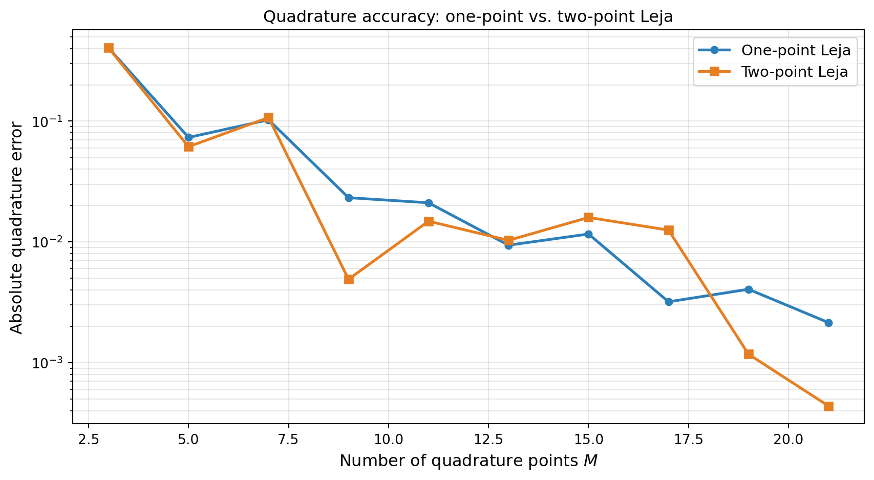

Figure 3: Quadrature error for one-point vs. two-point optimized Leja sequences. Two-point optimization improves accuracy for moderate M.

NoteWhen to Use Two-Point Optimization

Two-point Leja sequences are the default in PyApprox’s sparse grid framework because they produce more stable quadrature weights. The extra cost of solving a 2D optimization (vs. two 1D optimizations) is negligible compared to the function evaluations saved by better accuracy. Use TwoPointLejaObjective whenever quadrature accuracy matters — which is most practical applications.

Probability-Aware Leja for Non-Uniform Distributions

When the variable \(\theta\) follows a non-uniform distribution, we want the interpolant to be most accurate in the high-probability region. By choosing the orthogonal polynomial basis matched to the distribution, LejaSequence1D automatically concentrates nodes where the probability density is large.

For a \(\text{Beta}(\alpha, \beta)\) distribution on \([0, 1]\), the matched orthogonal polynomials are the Jacobi polynomials with parameters \((\beta - 1, \alpha - 1)\).

from scipy.stats import beta as beta_dist
from pyapprox.tutorial_figures._interpolation import plot_leja_beta

alpha_s, beta_s = 3.0, 5.0
rv_beta = beta_dist(alpha_s, beta_s)

# Uniform Leja on [-1, 1]  (Legendre = Jacobi(0,0))
poly_uniform = JacobiPolynomial1D(0.0, 0.0, bkd)
poly_uniform.set_nterms(30)
leja_uniform = LejaSequence1D(bkd, poly_uniform, ChristoffelWeighting(bkd), bounds=(-1.0, 1.0))

# Beta(3,5) Leja on [-1, 1] using matched Jacobi polynomials
# Jacobi params: (beta_param - 1, alpha_param - 1) = (4, 2)
poly_beta = JacobiPolynomial1D(beta_s - 1, alpha_s - 1, bkd)
poly_beta.set_nterms(30)
leja_beta = LejaSequence1D(bkd, poly_beta, ChristoffelWeighting(bkd), bounds=(-1.0, 1.0))

M = 12
nodes_uni, _ = leja_uniform.quadrature_rule(M)
nodes_beta_leja, _ = leja_beta.quadrature_rule(M)

# Map to [0, 1] for comparison with Beta PDF
nodes_uni_01 = (bkd.to_numpy(nodes_uni).ravel() + 1) / 2
nodes_beta_01 = (bkd.to_numpy(nodes_beta_leja).ravel() + 1) / 2

x_plot = np.linspace(0, 1, 300)

fig, axs = plt.subplots(2, 1, figsize=(11, 6), sharex=True)
plot_leja_beta(nodes_uni_01, nodes_beta_01, M, x_plot, rv_beta, axs)
plt.suptitle(f"Probability-aware Leja sequences, $M = {M}$", fontsize=12, y=1.01)
plt.tight_layout()
plt.show()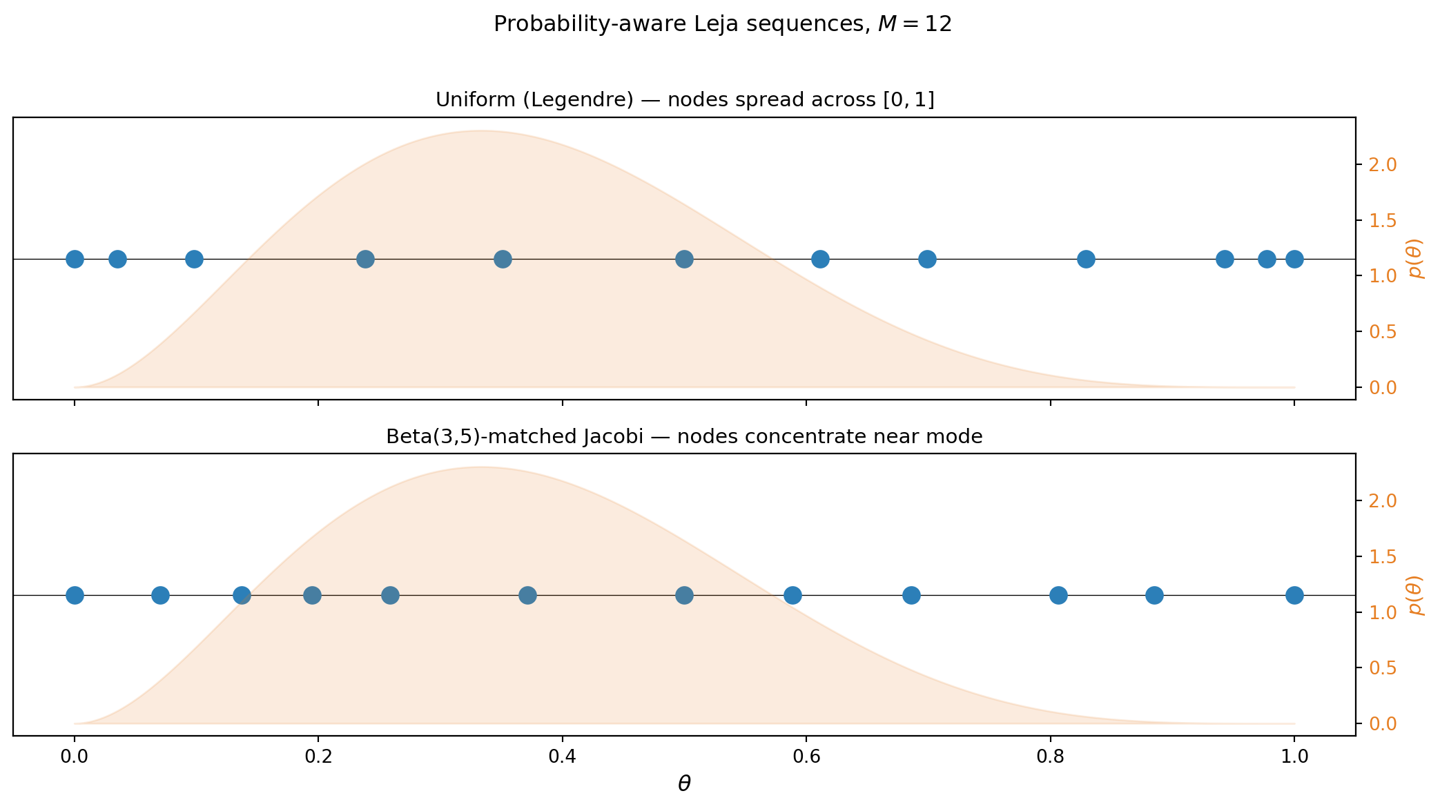

Figure 4: Leja sequences for uniform vs. Beta(3,5) matched polynomials. The Beta-matched sequence concentrates nodes toward the mode of the distribution.

The Beta-matched sequence places more nodes in the region where the Beta(3,5) distribution has its mass. This improves the interpolation accuracy of \(\mathbb{E}_\theta[f(\theta)]\) relative to a uniform Leja or CC sequence of the same size.

Key Takeaways

• Leja sequences are nested by construction: each point is added greedily and never discarded, so function evaluations are always reused as the sequence grows.
• The next Leja point maximizes a weighted distance product \(v(z) \prod_n |z - z^{(n)}|\); the Christoffel function weighting makes this near-optimal for polynomial interpolation.
• Two-point optimized Leja (TwoPointLejaObjective) adds points in pairs by maximizing a 2D determinant, producing more accurate quadrature weights than sequential one-point optimization.
• For analytic functions and a uniform distribution, Leja sequences match Clenshaw-Curtis in convergence rate while being more flexible (one point at a time, any growth pattern).
• LejaLagrangeFactory packages the Leja construction for direct use in sparse grid algorithms via create_basis_factories(..., basis_type="leja").
• Non-uniform distributions are handled by choosing JacobiPolynomial1D with parameters matched to the distribution, concentrating nodes in high-probability regions.

Exercises

NoteExercises

1. Nesting verification. Build a 5-point and a 10-point Leja sequence from the same seed. Verify that every point of the 5-point sequence appears in the 10-point sequence. Does this hold if you use Gauss-Legendre points instead?

2. Lebesgue constant. The Lebesgue constant \(\Lambda_M = \max_{x \in [-1,1]} \sum_j |\phi_j(x)|\) measures worst-case interpolation amplification. Compute \(\Lambda_M\) for \(M = 5, 10, 15\) for equidistant, CC, and Leja nodes. Which grows slowest?

3. Non-uniform convergence. Generate a Leja sequence matched to \(\theta \sim \text{Beta}(2, 8)\) and interpolate \(f(\theta) = \sin(10\theta)\). Compare the error in \(\mathbb{E}_\theta[f(\theta)]\) against a uniform Leja sequence of the same size.

4. Christoffel weighting. Replace the Christoffel weighting with PDFWeighting and compare the resulting node distribution. How does convergence change?

Next Steps

• Tensor Product Interpolation — Extend 1D interpolation to multiple dimensions using tensor products
• Isotropic Sparse Grids — Use Leja or CC nodes in the Smolyak combination scheme