
Design Under Uncertainty
PyApprox Tutorial Library
Optimize a cantilever beam’s cross-section under uncertain loads using deterministic and robust formulations.
TipDownload Notebook
Learning Objectives
After completing this tutorial, you will be able to:
- Formulate a deterministic constrained optimization problem using
ActiveSetFunctionandScipyTrustConstrOptimizer - Propagate uncertainty through a model using quadrature and assess failure probability at a deterministic optimum
- Build a robust optimization formulation using
SampleAverageConstraintwith mean + \(k \cdot \sigma\) risk measures - Compare deterministic and robust optimal designs in terms of cost and reliability
Prerequisites
Complete Forward UQ before this tutorial.
Problem Setup
We design the cross-section of a cantilever beam of length \(L = 100\) subject to uncertain tip loads \(X\) (horizontal) and \(Y\) (vertical). The beam has Young’s modulus \(E\) and yield stress \(R\), both uncertain. The design variables are the beam width \(w\) and depth \(t\).
The beam model returns two quantities of interest:
\[ \sigma = \frac{6L}{wt}\left(\frac{X}{w} + \frac{Y}{t}\right), \qquad D = \frac{4L^3}{Ewt}\sqrt{\frac{X^2}{w^4} + \frac{Y^2}{t^4}} \]
The design must satisfy two safety constraints: the stress must stay below the yield stress \(R\), and the displacement must stay below a threshold \(D_0 = 2.2535\):
\[ 1 - \frac{\sigma}{R} \geq 0, \qquad 1 - \frac{D}{D_0} \geq 0 \]
The objective is to minimize the cross-sectional area \(w \cdot t\).
import numpy as np
import matplotlib.pyplot as plt
from pyapprox.util.backends.numpy import NumpyBkd

bkd = NumpyBkd()
The Beam Model
We use CantileverBeam2DConstraints for the safety margin constraints and CantileverBeam2DObjective for the area objective. Both accept 6 input variables (X, Y, E, R, w, t) and provide analytical Jacobians.
from pyapprox_benchmarks.functions.algebraic.cantilever_beam_2d import (
    CantileverBeam2DAnalytical,
    CantileverBeam2DConstraints,
    CantileverBeam2DObjective,
)

beam = CantileverBeam2DAnalytical(length=100.0, bkd=bkd)
constraints_model = CantileverBeam2DConstraints(beam, yield_stress=40000.0, max_displacement=2.2535)
objective_model = CantileverBeam2DObjective(bkd)
Deterministic Optimization
First we solve a deterministic version: fix the uncertain variables at their nominal values and optimize \(w\) and \(t\) to minimize area subject to the safety constraints.
ActiveSetFunction fixes the non-design variables at nominal values and exposes only \(w\) and \(t\) to the optimizer. It dynamically propagates the Jacobian from the wrapped model, so the optimizer can use gradient information.
from pyapprox.interface.functions.marginalize import ActiveSetFunction

nominal_values = bkd.asarray([500.0, 1000.0, 2.9e7, 40000.0, 2.5, 3.0])
design_indices = [4, 5]  # w, t

det_objective = ActiveSetFunction(objective_model, nominal_values, design_indices, bkd)
det_constraints = ActiveSetFunction(constraints_model, nominal_values, design_indices, bkd)
Now set up and solve the optimization problem. The constraints must be \(\geq 0\) (feasibility), so we set lower bounds to 0 and upper bounds to \(\infty\).
from pyapprox.optimization.minimize.scipy.trust_constr import (
    ScipyTrustConstrOptimizer,
)
from pyapprox.optimization.minimize.constraints.protocols import (
    NonlinearConstraintProtocol,
)

# Wrap det_constraints as a NonlinearConstraintProtocol
class DetConstraintWrapper:
    def __init__(self, asf, bkd):
        self._asf = asf
        self._bkd = bkd
        # Dynamically bind jacobian if available
        if hasattr(asf, "jacobian"):
            self.jacobian = asf.jacobian

    def bkd(self):
        return self._bkd

    def nvars(self):
        return self._asf.nvars()

    def nqoi(self):
        return self._asf.nqoi()

    def __call__(self, sample):
        return self._asf(sample)

    def lb(self):
        return self._bkd.asarray([0.0, 0.0])

    def ub(self):
        return self._bkd.asarray([np.inf, np.inf])


det_con_wrapped = DetConstraintWrapper(det_constraints, bkd)

# Design variable bounds: w in [1, 10], t in [1, 10]
bounds = bkd.asarray([[1.0, 10.0], [1.0, 10.0]])
init_guess = bkd.asarray([[2.5], [3.0]])

optimizer = ScipyTrustConstrOptimizer(maxiter=200, gtol=1e-10)
optimizer.bind(det_objective, bounds, constraints=[det_con_wrapped])
det_result = optimizer.minimize(init_guess)

w_det = float(bkd.to_numpy(det_result.optima())[0, 0])
t_det = float(bkd.to_numpy(det_result.optima())[1, 0])
area_det = float(det_result.fun())
Propagating Uncertainty Through the Deterministic Optimum
The deterministic design assumes fixed nominal values for loads and material properties. In reality, \(X\), \(Y\), \(E\), and \(R\) are uncertain. Let us assess how the deterministic design performs under uncertainty by propagating random samples through the constraint model.
We model the uncertain variables as independent Gaussians:
| Variable | Mean | Std. Dev. |
|---|---|---|
| \(X\) (horizontal load) | 500 | 100 |
| \(Y\) (vertical load) | 1000 | 100 |
| \(E\) (Young’s modulus) | \(2.9 \times 10^7\) | \(1.45 \times 10^6\) |
| \(R\) (yield stress) | 40000 | 2000 |
from pyapprox.probability.univariate.gaussian import GaussianMarginal
from pyapprox.probability.joint.independent import IndependentJoint

marginals = [
    GaussianMarginal(mean=500.0, stdev=100.0, bkd=bkd),
    GaussianMarginal(mean=1000.0, stdev=100.0, bkd=bkd),
    GaussianMarginal(mean=2.9e7, stdev=1.45e6, bkd=bkd),
    GaussianMarginal(mean=40000.0, stdev=2000.0, bkd=bkd),
]
prior = IndependentJoint(marginals, bkd)

# Monte Carlo assessment at the deterministic optimum
np.random.seed(42)
N_mc = 10000
random_samples = prior.rvs(N_mc)  # (4, N_mc)

# Build full samples: random variables + fixed design
design_det = bkd.asarray([[w_det], [t_det]])
design_tiled = bkd.repeat(design_det, N_mc, axis=1)  # (2, N_mc)
full_samples = bkd.concatenate([random_samples, design_tiled], axis=0)

constraint_values = bkd.to_numpy(constraints_model(full_samples))  # (2, N_mc)

# Failure = either constraint < 0
stress_failures = np.sum(constraint_values[0, :] < 0)
disp_failures = np.sum(constraint_values[1, :] < 0)
any_failure = np.sum(np.any(constraint_values < 0, axis=0))
fig, axes = plt.subplots(1, 2, figsize=(12, 4))
labels = ["Stress constraint", "Displacement constraint"]
for ii, ax in enumerate(axes):
ax.hist(constraint_values[ii, :], bins=60, density=True, alpha=0.6,
color="#2C7FB8", edgecolor="k", lw=0.2)
ax.axvline(0, color="red", linestyle="--", lw=2, label="Failure boundary")
pct_fail = 100 * np.sum(constraint_values[ii, :] < 0) / N_mc
ax.set_xlabel(labels[ii])
ax.set_ylabel("Density")
ax.set_title(f"{pct_fail:.1f}% failure rate")
ax.legend()
ax.grid(True, alpha=0.2)
plt.tight_layout()
plt.show()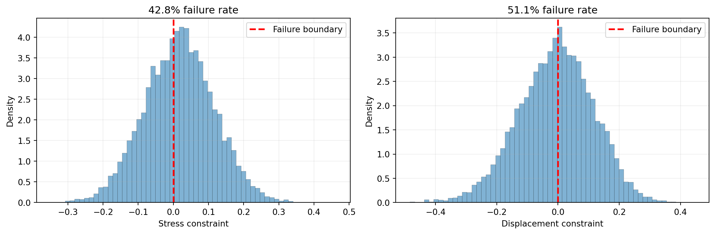
The deterministic design has a high failure rate because it was optimized assuming fixed (nominal) values for the uncertain variables. We need a robust formulation that accounts for uncertainty.
ImportantWhy deterministic optimization fails under uncertainty
The deterministic optimum pushes the design right to the constraint boundary at nominal conditions. Any perturbation in loads or material properties can push the design into the infeasible region. A robust formulation must include a safety margin.
Robust Optimization with Statistical Constraints
Instead of evaluating constraints at a single nominal point, we require that the mean minus a safety factor times the standard deviation of each constraint remains non-negative:
\[ \mathbb{E}[c_i(w, t)] - k \cdot \sigma[c_i(w, t)] \geq 0, \qquad i = 1, 2 \]
where the expectation and standard deviation are over the random variables \((X, Y, E, R)\), and \(k\) is a safety factor. This is equivalent to requiring \(\mu + k\sigma\) of the constraint violation to be non-positive, which ensures that the design remains feasible with high probability.
We compute the expectation using Gauss quadrature over the random variables. The SampleAverageConstraint class combines the model, quadrature rule, and statistical measure into a single constraint object.
from pyapprox.surrogates.quadrature.probability_measure_factory import (
    ProbabilityMeasureQuadratureFactory,
)

# Build quadrature rule for random variables (indices 0-3)
quad_factory = ProbabilityMeasureQuadratureFactory(
    marginals, [10, 10, 10, 10], bkd
)
quad_rule = quad_factory([0, 1, 2, 3])
quad_samples, quad_weights = quad_rule()

n_quad = quad_samples.shape[1]
from pyapprox.optimization.minimize.constraints.sample_average import (
SampleAverageConstraint,
)
from pyapprox.risk import SampleAverageMeanPlusStdev
# Use mean - 3*stdev >= 0, equivalently: -(mean + 3*stdev of negated constraint)
# But since our constraints are c_i >= 0, we want E[c_i] - k*std[c_i] >= 0.
# SampleAverageMeanPlusStdev computes mean + factor*stdev.
# So we use factor = -3 to get mean - 3*stdev.
safety_factor = 3
stat = SampleAverageMeanPlusStdev(-safety_factor, bkd)
robust_constraint = SampleAverageConstraint(
model=constraints_model,
quad_samples=quad_samples,
quad_weights=quad_weights,
stat=stat,
design_indices=[4, 5],
constraint_lb=bkd.asarray([0.0, 0.0]),
constraint_ub=bkd.asarray([np.inf, np.inf]),
bkd=bkd,
)Now solve the robust optimization problem. The objective is the same (minimize area), but we use ActiveSetFunction to reduce the objective to design variables only, and the SampleAverageConstraint enforces statistical feasibility.
robust_optimizer = ScipyTrustConstrOptimizer(maxiter=200, gtol=1e-10)
robust_optimizer.bind(det_objective, bounds, constraints=[robust_constraint])
robust_result = robust_optimizer.minimize(init_guess)

w_rob = float(bkd.to_numpy(robust_result.optima())[0, 0])
t_rob = float(bkd.to_numpy(robust_result.optima())[1, 0])
area_rob = float(robust_result.fun())
Comparing the Two Designs
# Propagate uncertainty at the robust optimum
design_rob = bkd.asarray([[w_rob], [t_rob]])
design_rob_tiled = bkd.repeat(design_rob, N_mc, axis=1)
full_samples_rob = bkd.concatenate([random_samples, design_rob_tiled], axis=0)

constraint_values_rob = bkd.to_numpy(constraints_model(full_samples_rob))
any_failure_rob = np.sum(np.any(constraint_values_rob < 0, axis=0))
from pyapprox_tutorials.figures import plot_duu_comparison
fig, axes = plt.subplots(1, 2, figsize=(12, 4))
plot_duu_comparison(constraint_values, constraint_values_rob, axes)
plt.tight_layout()
plt.show()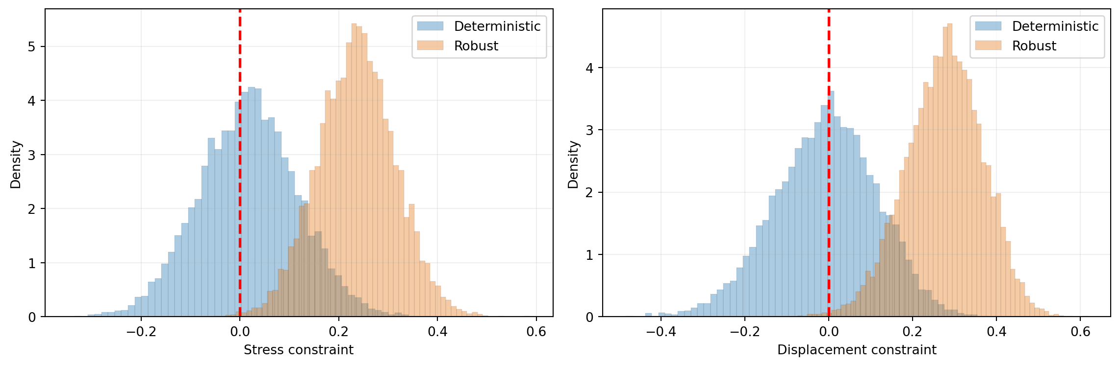
The robust design increases the cross-sectional area (cost) but dramatically reduces the failure probability by building in a safety margin against uncertainty.
Key Takeaways
- Deterministic optimization at nominal conditions pushes designs to constraint boundaries, leading to high failure rates under uncertainty
ActiveSetFunctionreduces a full model to design variables only, propagating Jacobians for gradient-based optimizationSampleAverageConstraintwraps a model with quadrature-based statistical constraints, combining anySampleStatistic(mean, mean\(\pm k\sigma\), CVaR) with the optimizer- The modular design lets you swap risk measures without changing the optimization setup — replace
SampleAverageMeanPlusStdevwithSampleAverageEntropicRiskorSampleAverageSmoothedAVaRfor alternative robustness criteria
Exercises
Change the safety factor from \(k = 3\) to \(k = 1\) and \(k = 5\). How does this affect the optimal area and failure probability? Plot the Pareto front (area vs. failure rate) for \(k \in \{0, 1, 2, 3, 4, 5\}\).
Replace
SampleAverageMeanPlusStdevwithSampleAverageMean(i.e., constrain only the expected constraint value). What happens to the failure rate? Why is mean-only insufficient?Increase the quadrature resolution from 10 to 20 points per dimension and compare the optimal design. Is the 10-point rule sufficiently accurate?
Next Steps
- Forward UQ — Propagate uncertainty through models using Monte Carlo and quadrature
- UQ with Polynomial Chaos — Build surrogates for efficient uncertainty propagation