import numpy as np
import matplotlib.pyplot as plt

from pyapprox.util.backends.numpy import NumpyBkd
from pyapprox.surrogates.sparsegrids import (
    IsotropicSparseGridFitter,
    TensorProductSubspaceFactory,
    LejaLagrangeFactory,
    compute_smolyak_coefficients,
    is_downward_closed,
)
from pyapprox.surrogates.affine.univariate import (
    LegendrePolynomial1D,
    LagrangeBasis1D,
)
from pyapprox.surrogates.affine.leja import (
    LejaSequence1D,
    ChristoffelWeighting,
)
from pyapprox.surrogates.affine.indices import (
    LinearGrowthRule,
    ClenshawCurtisGrowthRule,
)
from pyapprox.interface.functions.plot.plot2d_rectangular import (
    Plotter2DRectangularDomain,
    meshgrid_samples,
)
from pyapprox.interface.functions.fromcallable.function import (
    FunctionFromCallable,
)
from pyapprox.probability.univariate.uniform import UniformMarginal
from pyapprox_tutorials.figures._quadrature import (
    plot_smolyak_combo,
    plot_sg_points,
    plot_point_counts,
    plot_4d_convergence,
    plot_growth_rules,
)

bkd = NumpyBkd()
np.random.seed(42)

# Leja sequence for 1D bases (shared across cells)
marginal = UniformMarginal(-1.0, 1.0, bkd)
poly_leja = LegendrePolynomial1D(bkd)
poly_leja.set_nterms(30)
weighting = ChristoffelWeighting(bkd)
leja_seq = LejaSequence1D(bkd, poly_leja, weighting, bounds=(-1.0, 1.0))

# Shared factory — reusing one instance caches the Leja sequence,
# so all sparse grids in this tutorial avoid recomputing nodes.
leja_factory = LejaLagrangeFactory(marginal, bkd)Isotropic Sparse Grids: Breaking the Curse of Dimensionality
PyApprox Tutorial Library
Learn the Smolyak combination technique, construct isotropic sparse grids, compare point counts with tensor products, and study convergence theory.
TipDownload Notebook
Learning Objectives
After completing this tutorial, you will be able to:
- Explain the Smolyak combination technique and its relationship to tensor products
- Define downward-closed index sets and compute Smolyak coefficients
- Construct isotropic sparse grids using
IsotropicSparseGridFitter - Compare sparse grid point counts with tensor product grids across dimensions
- Measure sparse grid convergence against the theoretical rate \(N^{-r}(\log N)^{(r+2)(D-1)+1}\)
- Compute statistics via
surrogate.mean()
Prerequisites
Complete Tensor Product Interpolation before this tutorial. You should understand tensor product grids, the curse of dimensionality, and 1D Lagrange interpolation.
Setup
The Smolyak Combination Technique
The key observation behind sparse grids is that a \(D\)-dimensional function can be approximated by a linear combination of low-order tensor product interpolants. Let \(f_\beta\) denote the tensor product interpolant indexed by \(\beta \in \mathbb{Z}_{\geq 0}^D\), where \(\beta_i\) controls the refinement level in dimension \(i\). The Smolyak approximation is
\[ f_{\mathcal{I}}(\mathbf{z}) = \sum_{\beta \in \mathcal{I}} c_\beta\, f_\beta(\mathbf{z}), \]
where \(\mathcal{I}\) is an index set and \(c_\beta\) are Smolyak coefficients. The index set \(\mathcal{I}\) controls which tensor product components are included, and the coefficients \(c_\beta\) are chosen so that the combination reproduces the full tensor product exactly in the limit.
Downward-Closed Index Sets
For the combination formula to be valid, \(\mathcal{I}\) must be downward closed (also called admissible):
\[ \gamma \leq \beta \text{ (entry-wise) and } \beta \in \mathcal{I} \implies \gamma \in \mathcal{I}. \]
Intuitively, you cannot include a high-resolution sub-grid in dimension \(i\) without also including all coarser sub-grids.
# Example: 2D isotropic index set at level l=2
# I(2) = {β : ||β||_1 ≤ 2}
indices_valid = bkd.asarray(
    [[0, 0, 1, 0, 1, 2], [0, 1, 0, 2, 1, 0]]
)
# Missing (1,0) — not downward closed
indices_invalid = bkd.asarray(
    [[0, 0, 2], [0, 2, 2]]
)

is_downward_closed(indices_valid, bkd)
is_downward_closed(indices_invalid, bkd)FalseSmolyak Coefficients
For a downward-closed index set the Smolyak coefficient of \(\beta\) is
\[ c_\beta = \sum_{\substack{i \in \{0,1\}^D \\ \beta + i \in \mathcal{I}}} (-1)^{\lVert i \rVert_1}. \]
For the isotropic index set \(\mathcal{I}(l) = \{\beta : \lVert \beta \rVert_1 \leq l\}\) with level \(l\) and \(D\) dimensions, the coefficients alternate in sign and their magnitudes are given by binomial coefficients. A key property is that the coefficients always sum to 1.
coefs = compute_smolyak_coefficients(indices_valid, bkd)Visualizing the Combination Structure
The figure below shows the tensor product subspaces that enter the \(l = 2\) isotropic sparse grid in 2D. Each sub-grid is drawn as a contour plot of the corresponding interpolant, with its Smolyak coefficient labelled. Sub-grids with coefficient \(+1\) are added; those with coefficient \(-1\) are subtracted.
from pyapprox.surrogates.tensorproduct import TensorProductInterpolant

def target_2d(samples):
    """cos(π z₁) cos(π z₂/2), shape (1, N)."""
    return bkd.reshape(
        bkd.cos(np.pi * samples[0]) * bkd.cos(np.pi * samples[1] / 2),
        (1, -1),
    )

max_level = 2
growth = ClenshawCurtisGrowthRule()

# Indices and coefficients for the isotropic set
iso_indices = indices_valid  # already level=2 set
iso_coefs = compute_smolyak_coefficients(iso_indices, bkd)

# Evaluation grid for contour plots
x_plot = np.linspace(-1, 1, 41)
X_plot, Y_plot = np.meshgrid(x_plot, x_plot)
eval_pts = bkd.asarray(np.vstack([X_plot.ravel(), Y_plot.ravel()]))

# Pre-compute tensor product interpolants for each sub-grid
tp_interpolants = {}
for ii in range(max_level + 1):
    for jj in range(max_level + 1):
        if ii + jj > max_level:
            continue
        npts = [growth(ii), growth(jj)]
        bases_1d = [
            LagrangeBasis1D(bkd, leja_seq.quadrature_rule),
            LagrangeBasis1D(bkd, leja_seq.quadrature_rule),
        ]
        tp = TensorProductInterpolant(bkd, bases_1d, npts)
        tp_samples = tp.get_samples()
        tp.set_values(target_2d(tp_samples))
        Z = bkd.to_numpy(tp(eval_pts)).reshape(X_plot.shape)
        sg = bkd.to_numpy(tp_samples)
        tp_interpolants[(ii, jj)] = (Z, sg)

fig, axs = plt.subplots(
    max_level + 1, max_level + 1,
    figsize=((max_level + 1) * 4, (max_level + 1) * 3.5),
)
plot_smolyak_combo(
    fig, axs, max_level, iso_indices, iso_coefs,
    eval_pts, X_plot, Y_plot, tp_interpolants,
)
plt.tight_layout()
plt.show()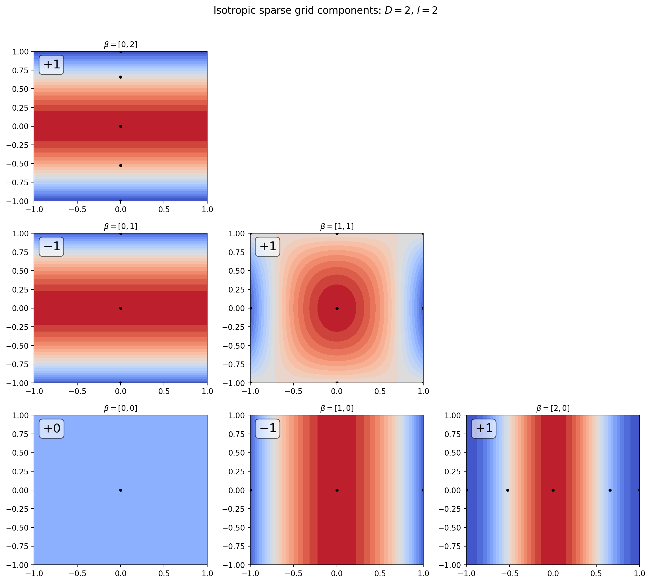
Building an Isotropic Sparse Grid
The sparse grid combines these tensor product subspaces automatically. We create one by specifying basis factories (which know how to build 1D bases at any resolution), a growth rule (mapping level \(\ell\) to the number of 1D nodes \(M_\ell\)), and a level (the maximum \(L^1\) norm of multi-indices).
The new fitter API separates construction from evaluation:
- Create a
TensorProductSubspaceFactoryfrom your factories and growth rule - Create an
IsotropicSparseGridFitterwith the factory and level - Call
get_samples()to get the sample locations - Evaluate your function at those locations
- Call
fit(values)to get the result containing the surrogate
nvars = 2
factories = [leja_factory] * nvars
growth = ClenshawCurtisGrowthRule()

# Create isotropic sparse grids at increasing levels
for level in range(5):
    tp_factory = TensorProductSubspaceFactory(bkd, factories, growth)
    fitter = IsotropicSparseGridFitter(bkd, tp_factory, level)
    samples = fitter.get_samples()
    nsamples = samples.shape[1]
    # Fit with dummy values to get subspace count
    values = bkd.ones((1, nsamples))
    result = fitter.fit(values)
Visualizing Sparse Grid Points
levels_list = [0, 1, 2, 3]
sample_arrays = []
nsamples_list = []
for level in levels_list:
    tp_factory = TensorProductSubspaceFactory(bkd, factories, growth)
    fitter = IsotropicSparseGridFitter(bkd, tp_factory, level)
    samples = bkd.to_numpy(fitter.get_samples())
    sample_arrays.append(samples)
    nsamples_list.append(samples.shape[1])

fig, axes = plt.subplots(1, 4, figsize=(14, 3.5))
plot_sg_points(axes, levels_list, sample_arrays, nsamples_list)
plt.tight_layout()
plt.show()
Interpolating a 2D Function
Let us interpolate \(f(z_1, z_2) = \cos(\pi z_1)\cos(\pi z_2/2)\) on \([-1,1]^2\) and compare with a tensor product of the same level.
def target_function(samples, bkd):
    z1, z2 = samples[0, :], samples[1, :]
    values = bkd.cos(np.pi * z1) * bkd.cos(np.pi * z2 / 2)
    return bkd.reshape(values, (1, -1))

level = 3
tp_factory = TensorProductSubspaceFactory(bkd, factories, growth)
fitter = IsotropicSparseGridFitter(bkd, tp_factory, level)
samples = fitter.get_samples()
values = target_function(samples, bkd)
result = fitter.fit(values)
surrogate = result.surrogate

# Compare point counts with tensor product at same level
nsamples = samples.shape[1]

# Wrap true function for plotting
true_func = FunctionFromCallable(
    nqoi=1, nvars=2,
    fun=lambda s: target_function(s, bkd),
    bkd=bkd,
)

fig, axes = plt.subplots(1, 3, figsize=(15, 4))
plot_limits = [-1, 1, -1, 1]

# True function
true_plotter = Plotter2DRectangularDomain(true_func, plot_limits)
true_plotter.plot_contours(axes[0], qoi=0, npts_1d=51, levels=20, cmap="coolwarm")
axes[0].set_title("True function")
axes[0].set_xlabel("$z_1$")
axes[0].set_ylabel("$z_2$")

# Sparse grid interpolant
sg_plotter = Plotter2DRectangularDomain(surrogate, plot_limits)
sg_plotter.plot_contours(axes[1], qoi=0, npts_1d=51, levels=20, cmap="coolwarm")
sg_pts = bkd.to_numpy(samples)
axes[1].scatter(sg_pts[0], sg_pts[1], c="k", s=20, alpha=0.7)
axes[1].set_title(f"Sparse grid ({nsamples} pts)")
axes[1].set_xlabel("$z_1$")

# Error plot
X, Y, eval_pts = meshgrid_samples(51, plot_limits, bkd)
true_vals = target_function(eval_pts, bkd)
approx_vals = surrogate(eval_pts)
error_vals = bkd.abs(true_vals - approx_vals)
error_2d = bkd.reshape(error_vals[0], X.shape)
im_err = axes[2].contourf(
    bkd.to_numpy(X), bkd.to_numpy(Y), bkd.to_numpy(error_2d),
    levels=20, cmap="Reds",
)
axes[2].set_title(f"|Error| (max={float(bkd.max(error_vals)):.2e})")
axes[2].set_xlabel("$z_1$")
plt.colorbar(im_err, ax=axes[2])

plt.tight_layout()
plt.show()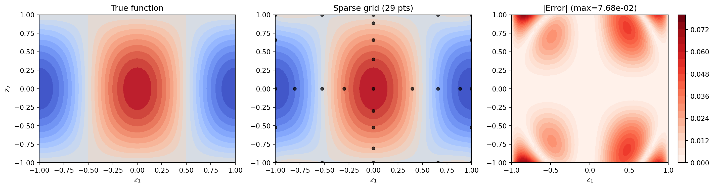
Point Count Comparison
The sparse grid’s main advantage is dramatically fewer points than tensor products in moderate-to-high dimensions.
dims_compare = [2, 5, 10]
max_levels = {2: 5, 5: 5, 10: 4}

levels_data, sg_counts_data, tp_counts_data = [], [], []
for d in dims_compare:
    levels_range = np.arange(0, max_levels[d] + 1)
    sg_counts, tp_counts = [], []
    for ell in levels_range:
        facs_d = [leja_factory] * d
        tp_fac = TensorProductSubspaceFactory(bkd, facs_d, growth)
        fitter = IsotropicSparseGridFitter(bkd, tp_fac, int(ell))
        sg_counts.append(fitter.get_samples().shape[1])
        tp_counts.append(growth(int(ell)) ** d)
    levels_data.append(levels_range)
    sg_counts_data.append(sg_counts)
    tp_counts_data.append(tp_counts)

fig, axs = plt.subplots(1, 3, figsize=(14, 5), sharey=False)
plot_point_counts(axs, dims_compare, levels_data, sg_counts_data, tp_counts_data)
plt.suptitle(
    "Sparse grid vs. tensor product: point count scaling", fontsize=13
)
plt.tight_layout()
plt.show()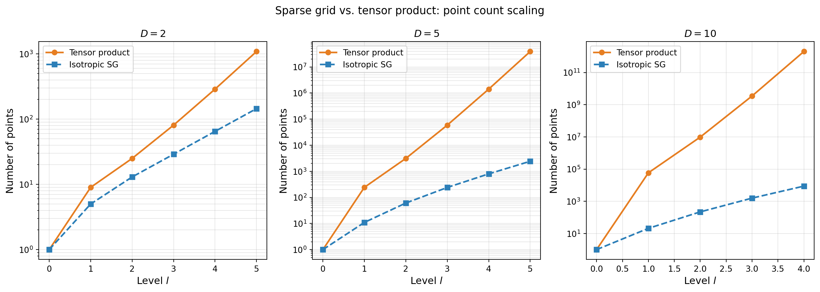
The table below shows the exact counts. Tensor product counts are computed analytically as \(M_\ell^D\); sparse grid counts are measured from actual grid construction.
Convergence Study: 4D Function
The isotropic sparse grid convergence theorem (Barthelmann et al. 2000) states that for a function with \(r\) continuous mixed derivatives and \(M_{\mathcal{I}}\) sparse grid points:
\[ \lVert f - f_{\mathcal{I}}\rVert_{\infty} \leq C_{D,r}\, M_{\mathcal{I}}^{-r}\,(\log M_{\mathcal{I}})^{(r+2)(D-1)+1}. \]
Compare this to the tensor product rate \(M^{-r/D}\): the sparse grid replaces the \(1/D\) exponent with a logarithmic correction. For large \(D\) and smooth \(f\), this is a dramatic improvement.
nvars4 = 4

def fun4d(samples, bkd):
    """Smooth 4D function. Returns shape (1, nsamples)."""
    shifted = (samples + 1) / 2 - 0.5
    return bkd.reshape(
        bkd.exp(-0.05 * bkd.sum(shifted ** 2, axis=0)), (1, -1)
    )

# Validation samples
validation_samples = bkd.asarray(np.random.uniform(-1, 1, (nvars4, 1000)))
validation_values = fun4d(validation_samples, bkd)

# Sparse grid convergence
sg_npts, sg_errors = [], []
for level in range(5):
    facs4 = [leja_factory] * nvars4
    tp_fac4 = TensorProductSubspaceFactory(bkd, facs4, growth)
    fitter = IsotropicSparseGridFitter(bkd, tp_fac4, level)
    samples = fitter.get_samples()
    result = fitter.fit(fun4d(samples, bkd))

    approx = result.surrogate(validation_samples)
    err = float(
        bkd.sqrt(bkd.sum((validation_values - approx) ** 2))
        / np.sqrt(1000)
    )
    sg_npts.append(samples.shape[1])
    sg_errors.append(err)

# Tensor product convergence (only small levels feasible)
tp_npts, tp_errors = [], []
for level in range(4):
    n_tp = growth(level) ** nvars4
    if n_tp > 200_000:
        break

    tp_bases = [
        LagrangeBasis1D(bkd, leja_seq.quadrature_rule)
        for _ in range(nvars4)
    ]
    nterms = [growth(level)] * nvars4
    tp = TensorProductInterpolant(bkd, tp_bases, nterms)
    tp_samples = tp.get_samples()
    tp.set_values(fun4d(tp_samples, bkd))

    approx = tp(validation_samples)
    err = float(
        bkd.sqrt(bkd.sum((validation_values - approx) ** 2))
        / np.sqrt(1000)
    )
    tp_npts.append(n_tp)
    tp_errors.append(err)

fig, ax = plt.subplots(figsize=(8, 5))
plot_4d_convergence(ax, sg_npts, sg_errors, tp_npts, tp_errors)
plt.tight_layout()
plt.show()
Growth Rules
The growth rule maps a level \(\ell\) to the number of quadrature nodes \(M_\ell\) used in that dimension at that level. The choice affects the total point count and the nesting properties of the grid.
| Rule | Formula | Example (l=0,1,2,3,4) |
|---|---|---|
| Linear | \(M_0 = 1\); \(M_\ell = 2\ell+1\) | 1, 3, 5, 7, 9 |
| Clenshaw-Curtis | \(M_0 = 1\); \(M_\ell = 2^\ell+1\) | 1, 3, 5, 9, 17 |
linear = LinearGrowthRule(scale=2, shift=1)
cc = ClenshawCurtisGrowthRule()

levels_gr = np.arange(0, 11)
rules_data = [
    ("Linear ($2\\ell+1$)", [linear(int(ell)) for ell in levels_gr]),
    ("CC ($2^\\ell+1$)", [cc(int(ell)) for ell in levels_gr]),
]

fig, ax = plt.subplots(figsize=(8, 4))
plot_growth_rules(ax, levels_gr, rules_data)
plt.tight_layout()
plt.show()
Computing Statistics with surrogate.mean()
Sparse grids double as quadrature rules: the combination of 1D quadrature weights yields multivariate weights that integrate polynomials of the appropriate mixed degree exactly. The surrogate.mean() method returns \(\mathbb{E}[f(\mathbf{Z})]\) for the measure determined by the 1D bases.
# Compute E[cos(πZ₁)cos(πZ₂/2)] over U(-1,1)²
# Exact: (1/4)∫cos(πz₁)dz₁ · ∫cos(πz₂/2)dz₂ = (1/4)·0·(4/π) = 0
# because ∫_{-1}^{1} cos(πz₁) dz₁ = [sin(πz₁)/π]_{-1}^{1} = 0
exact_mean = 0.0

tp_factory_quad = TensorProductSubspaceFactory(bkd, factories, growth)
fitter_quad = IsotropicSparseGridFitter(bkd, tp_factory_quad, level=4)
samples_quad = fitter_quad.get_samples()
values_quad = target_function(samples_quad, bkd)
result_quad = fitter_quad.fit(values_quad)
nsamples_quad = samples_quad.shape[1]

sg_mean = float(result_quad.surrogate.mean()[0])
Summary
- The Smolyak sparse grid is a linear combination of low-order tensor product interpolants indexed by a downward-closed index set; the combination cancels high-order cross-terms that contribute little accuracy.
- Smolyak coefficients alternate in sign; their sum over any downward-closed index set equals 1.
- For \(D\) dimensions and \(r\) mixed derivatives, the sparse grid error satisfies \(O(N^{-r}(\log N)^{(r+2)(D-1)+1})\) vs. \(O(N^{-r/D})\) for tensor products.
- The growth rule (linear, Clenshaw-Curtis, exponential) controls how rapidly the 1D node count grows with level. Certain quadrature rules demand specific growth patterns (e.g. Clenshaw-Curtis requires Clenshaw-Curtis growth), while faster growth adds larger subspace grids at each new level, enabling greater parallelism of function evaluations in adaptive settings.
surrogate.mean()provides a direct route to computing \(\mathbb{E}[f]\) without additional sampling.
Exercises
NoteExercises
Coefficient verification. For \(D = 3\), \(l = 3\), build the isotropic index set and compute the Smolyak coefficients using
compute_smolyak_coefficients. Verify that they sum to 1.Growth rule impact. Build two 2D isotropic sparse grids at \(l = 4\), one with
LinearGrowthRule(scale=2, shift=1)and one withClenshawCurtisGrowthRule(). Compare point counts and interpolation errors for \(f(z_1,z_2) = \exp(-z_1^2 - z_2^2)\).High dimensions. For \(D = 6\) and \(l = 3\), compute the sparse grid and tensor product point counts. What is the ratio?
Statistics. Use
surrogate.mean()to compute \(\mathbb{E}[\cos(\pi z_1)\cos(\pi z_2/2)]\) over \(\mathcal{U}(-1,1)^2\). Compare with the known analytic value (which is 0, by symmetry of cosine over \([-1,1]\)).
Next Steps
- UQ with Sparse Grids — Compute Sobol indices, covariance, and marginal densities from sparse grids via SG-to-PCE conversion
- Adaptive Sparse Grids — Anisotropic functions can be resolved even more efficiently by adapting the index set to the data
- Multifidelity Sparse Grids — Combine sparse grids across a hierarchy of model fidelities