Not All Experiments Are Equal: Introduction to Experimental Design
PyApprox Tutorial Library
How sensor placement affects what we learn about uncertain parameters.
TipDownload Notebook
Learning Objectives
After completing this tutorial, you will be able to:
- Explain why different sensor placements produce different posterior distributions
- Connect the sensitivity structure of the model to the direction of posterior uncertainty reduction
- Compare experimental designs by their posterior covariance
- Define Expected Information Gain (EIG) and compute it for linear Gaussian problems
- Identify optimal single-sensor and two-sensor placements for the cantilever beam
Prerequisites
Complete From Data to Parameters: Introduction to Bayesian Inference before this tutorial.
The Setup: Uncertain Loading on a Known Beam
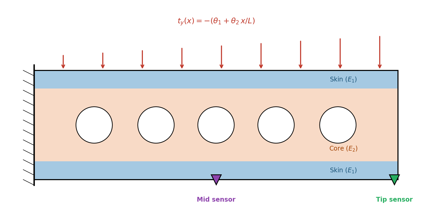
We return to the composite cantilever beam from the opening tutorial, but now the material properties are known and the applied load is uncertain. The traction on the top surface is:
\[ t_y(x;\, \theta_1, \theta_2) = -(\theta_1 + \theta_2\, x / L) \]
where \(\theta_1\) is the constant component and \(\theta_2\) controls the slope. We want to learn \((\theta_1, \theta_2)\) from deflection measurements. The question is: where on the beam should we place a sensor?
Figure 1 shows the physical setup: the composite beam clamped at the left, with the uncertain distributed load on top and two candidate sensor locations.
Same Budget, Different Answers
Suppose we have budget for exactly one deflection measurement. We can place the sensor at the tip or at the midpoint. Both cost the same. Both produce a single number. But they lead to different conclusions about \((\theta_1, \theta_2)\).
To see this, we set up the problem and compute the exact posterior for each sensor placement.
Figure 2 shows the result. The prior is the same broad ellipse in both cases, but the two sensors produce posteriors that are elongated in different directions.
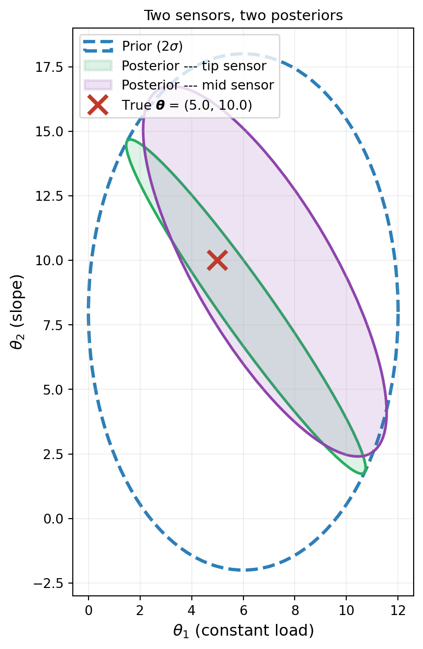
This is the key observation: the same data budget produces different posteriors depending on where we measure. Each sensor constrains a different combination of \(\theta_1\) and \(\theta_2\), leaving a different direction unresolved. The choice of experiment determines what we learn.
Why Are They Different?
The answer lies in the sensitivity of each measurement to the two parameters. The deflection at any location \(x_s\) is a linear function of \((\theta_1, \theta_2)\):
\[ \delta(x_s) = a_1(x_s)\, \theta_1 + a_2(x_s)\, \theta_2 \]
The coefficients \(a_1\) and \(a_2\) encode how strongly the measurement at \(x_s\) responds to each parameter. Figure 3 shows the deflection as a function of \((\theta_1, \theta_2)\) for the two sensor locations. The contour orientation determines which parameter direction the measurement constrains.

The contours are straight lines (the model is linear), but they have different slopes at the two locations. This means the two sensors provide constraints along different directions in parameter space — exactly what we saw in the posterior ellipses.
The Observation Matrix
Because linear elasticity is linear in the applied load, the deflection at any sensor location \(x_s\) satisfies:
\[ \delta(x_s) = \underbrace{[a_1(x_s),\; a_2(x_s)]}_{\mathbf{a}(x_s)^\top} \begin{bmatrix} \theta_1 \\ \theta_2 \end{bmatrix} \]
We compute the sensitivity vector \(\mathbf{a}(x_s)\) by superposition: solve the FEM once with a unit constant load (\(\theta_1 = 1\), \(\theta_2 = 0\)) and once with a unit slope load (\(\theta_1 = 0\), \(\theta_2 = 1\)). The deflections from these two solves give \(a_1(x_s)\) and \(a_2(x_s)\) directly.
The ratio \(a_2 / a_1\) determines the contour slope in Figure 3. Different ratios mean different constraint directions, which is why the posteriors differ.
Which Sensor Learned More?
Both sensors reduced the posterior uncertainty compared to the prior, but by different amounts. We quantify this by comparing the posterior covariance. A smaller covariance means the experiment was more informative.
def cov_det(gaussian):
    return bkd.to_float(bkd.det(gaussian.covariance()))

def cov_std(gaussian, idx):
    return bkd.to_float(bkd.sqrt(gaussian.covariance()[idx, idx]))
The determinant of the posterior covariance measures the “volume” of the uncertainty ellipse. A smaller determinant means the experiment squeezed the ellipse into a smaller area.
Combining Sensors: Signal Strength vs. Diversity
Suppose we have budget for two sensors. Should we place both at the tip (maximizing signal strength), or one at the tip and one at the midpoint (diversifying)?
With two sensors, the observation model becomes:
\[ \begin{bmatrix} \delta(x_1) \\ \delta(x_2) \end{bmatrix} = \begin{bmatrix} \mathbf{a}(x_1)^\top \\ \mathbf{a}(x_2)^\top \end{bmatrix} \begin{bmatrix} \theta_1 \\ \theta_2 \end{bmatrix} + \begin{bmatrix} \varepsilon_1 \\ \varepsilon_2 \end{bmatrix} \]
Figure 4 compares three configurations: two sensors at the tip, two at the midpoint, and one at each.
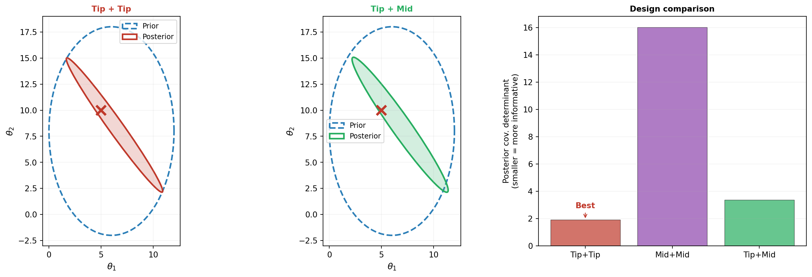
The result may be surprising: two sensors at the tip beat the mixed placement. Why? For this beam, the sensitivity directions at the tip and midpoint are nearly identical — both sensors constrain almost the same parameter combination. The midpoint simply has a weaker signal (smaller deflection). The repeated tip measurement averages out observation noise, extracting more information from the strong signal. Replacing one strong tip measurement with a weaker midpoint measurement trades noise-averaging ability for negligible diversity.
The determinants confirm the bar chart: Tip+Tip produces the tightest posterior. This illustrates an important nuance: diversification only helps when the sensors provide genuinely complementary information — that is, when their sensitivity directions differ substantially. When all candidate locations “see” the parameters through nearly the same linear combination, placing sensors where the signal is strongest wins. The two-sensor EIG heatmap below confirms this.
Expected Information Gain
So far we’ve compared designs after collecting data. But we want to choose the design before running the experiment. The observation is random (because of noise), so we need a measure of informativeness that averages over possible outcomes.
The Expected Information Gain (EIG) does exactly this:
\[ \text{EIG}(\xi) = \mathbb{E}_{y \mid \xi}\!\big[\text{KL}\!\left(p(\boldsymbol{\theta} \mid y, \xi) \;\|\; p(\boldsymbol{\theta})\right)\big] \]
The KL divergence measures how much the posterior differs from the prior — how much the experiment “taught” us. The expectation averages over all possible data \(y\) we might observe. Higher EIG means the design is expected to be more informative, regardless of what data actually arrives.
For our linear Gaussian problem, the EIG has a closed form that we can compute using DenseGaussianConjugatePosterior:
def compute_eig(A_design):
    """Expected Information Gain for linear Gaussian model."""
    nobs = A_design.shape[0]
    noise_cov = bkd.eye(nobs) * sigma_noise**2
    post = DenseGaussianConjugatePosterior(
        bkd.asarray(A_design),
        prior_mean,
        prior_cov,
        noise_cov,
        bkd,
    )
    dummy_obs = bkd.zeros((nobs, 1))
    post.compute(dummy_obs)
    return post.expected_kl_divergence()

# Single-sensor EIG
eig_tip = compute_eig(a_tip.reshape(1, -1))
eig_mid = compute_eig(a_mid.reshape(1, -1))
NoteEIG depends on the design, not the data
The EIG for the linear Gaussian case involves only \(\mathbf{A}\), \(\boldsymbol{\Sigma}_{\text{prior}}\), and \(\sigma_{\text{noise}}\) — it doesn’t depend on the observation \(y\). This means we can compare designs without running any experiments. For nonlinear models, the EIG generally depends on the data and must be estimated by simulation, which is more expensive.
Sensor Placement Sweep
With EIG as our design criterion, we can systematically search over all candidate sensor locations. Figure 5 shows the EIG as a function of sensor position along the beam.

Two-Sensor Optimization
For two sensors, we search over all pairs \((x_1, x_2)\). Figure 6 shows the EIG as a heatmap. The off-diagonal maxima confirm the complementarity principle: the best pair places sensors at different locations.

Key Takeaways
- Different experiments produce different posteriors, even with the same prior and data budget. The choice of experiment determines what we learn.
- The sensitivity structure of the model (encoded in the observation matrix \(\mathbf{A}\)) determines which parameter directions a measurement constrains. The posterior ellipse is elongated in the unconstrained direction.
- Diversification only helps when sensors provide genuinely different information. When sensitivity directions are similar across locations, concentrating measurements where the signal is strongest can outperform diversifying to weaker locations.
- Expected Information Gain provides a principled, data-independent measure of design quality. For linear Gaussian problems, it has a closed-form expression.
- The sensor placement problem is a concrete instance of experimental design: the optimal locations are those that maximize the expected information about the parameters.
Exercises
Add a third sensor location at \(x = L/4\) (quarter-span). Compute its EIG and compare to tip and midpoint. Where does it rank?
Change the prior to be correlated: \(\Sigma_{\text{prior}} = \begin{bmatrix} 9 & 6 \\ 6 & 25 \end{bmatrix}\). How do the posterior ellipses change? Does the optimal sensor location change?
Increase the noise level by a factor of 5. How does the EIG sweep change? Does the optimal location shift, or just the overall EIG scale?
(Challenge) Find the optimal three-sensor placement by exhaustive search over a grid. Is the gain from 2 to 3 sensors as large as from 1 to 2? Plot the posterior ellipse for the optimal triple.
Next Steps
Continue with:
- Bayesian Optimal Experimental Design — Systematic optimization of experiments using EIG