Approximate Control Variate Monte Carlo
PyApprox Tutorial Library
Extending control variates to the practical case where the low-fidelity model statistic is unknown, using additional low-fidelity samples in its place.
TipDownload Notebook
Learning Objectives
After completing this tutorial, you will be able to:
- Explain why an unknown low-fidelity mean undermines the CVMC correction
- Write down the Approximate Control Variate (ACV) estimator and describe its two sample sets
- Explain how the ratio \(r\) of low-fidelity to high-fidelity samples controls variance reduction
- Identify the limit in which ACV recovers the full CVMC variance reduction
Prerequisites
Complete Control Variate Monte Carlo before this tutorial.
The Problem: CVMC Needs a Number We Don’t Have
The CVMC estimator corrects the high-fidelity (HF) mean estimate using
\[ \hat{\mu}_\alpha^{\text{CV}} = \hat{\mu}_\alpha + \eta \left(\hat{\mu}_\kappa - \mu_\kappa\right). \]
The correction term \(\hat{\mu}_\kappa - \mu_\kappa\) works because \(\mu_\kappa\) is a fixed number: the true low-fidelity (LF) mean. Subtracting it centers the LF estimator error at zero, so the correction has mean zero and purely cancels correlated HF error.
For a practical numerical model, \(\mu_\kappa\) is almost never known analytically. The natural instinct is to estimate it from samples. But this creates a problem: if we use the same \(N\) samples to estimate both \(\hat{\mu}_\alpha\) and \(\hat{\mu}_\kappa\), the correction term becomes \(\hat{\mu}_\kappa(\mathcal{Z}_N) - \hat{\mu}_\kappa(\mathcal{Z}_N) = 0\) — it vanishes identically and we gain nothing.
If instead we use a separate set of LF samples to estimate \(\mu_\kappa\), the correction is no longer zero but it is now noisy — we are using one random quantity to cancel another. How noisy it is depends on how many LF samples we use.
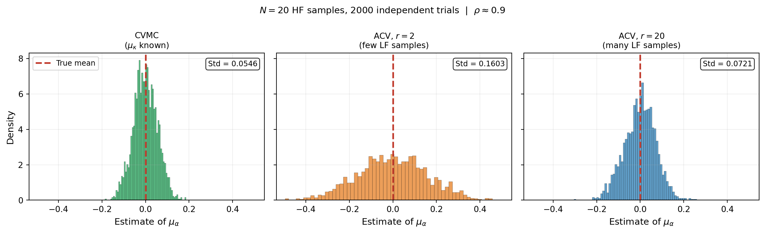
Figure 1 makes this concrete. Each panel shows the distribution of the corrected estimator when \(\mu_\kappa\) is: (left) known exactly, (centre) estimated from a small LF sample, (right) estimated from a large LF sample.
The figure shows the core trade-off clearly. A noisy correction (centre) is better than no correction at all — it still reduces variance compared to plain MC — but it cannot match the precision of CVMC. A cheap LF model means we can afford large \(r\), closing the gap to CVMC at modest extra cost.
The ACV Estimator
Approximate Control Variate Monte Carlo (ACVMC) [GGEJJCP2020] formalises this idea. Let \(\mathcal{Z}_N\) be the \(N\) samples shared by both models, and let \(\mathcal{Z}_{rN} \supset \mathcal{Z}_N\) be the larger set of \(rN\) samples used only for \(f_\kappa\). The ACV estimator is
\[ \hat{\mu}_\alpha^{\text{ACV}} = \hat{\mu}_\alpha(\mathcal{Z}_N) + \eta \Bigl(\hat{\mu}_\kappa(\mathcal{Z}_N) - \hat{\mu}_\kappa(\mathcal{Z}_{rN})\Bigr). \tag{1}\]
The true \(\mu_\kappa\) never appears: it cancels in expectation because both LF estimates are unbiased for the same quantity. The estimator is unbiased for any \(r > 1\) and any \(\eta\).
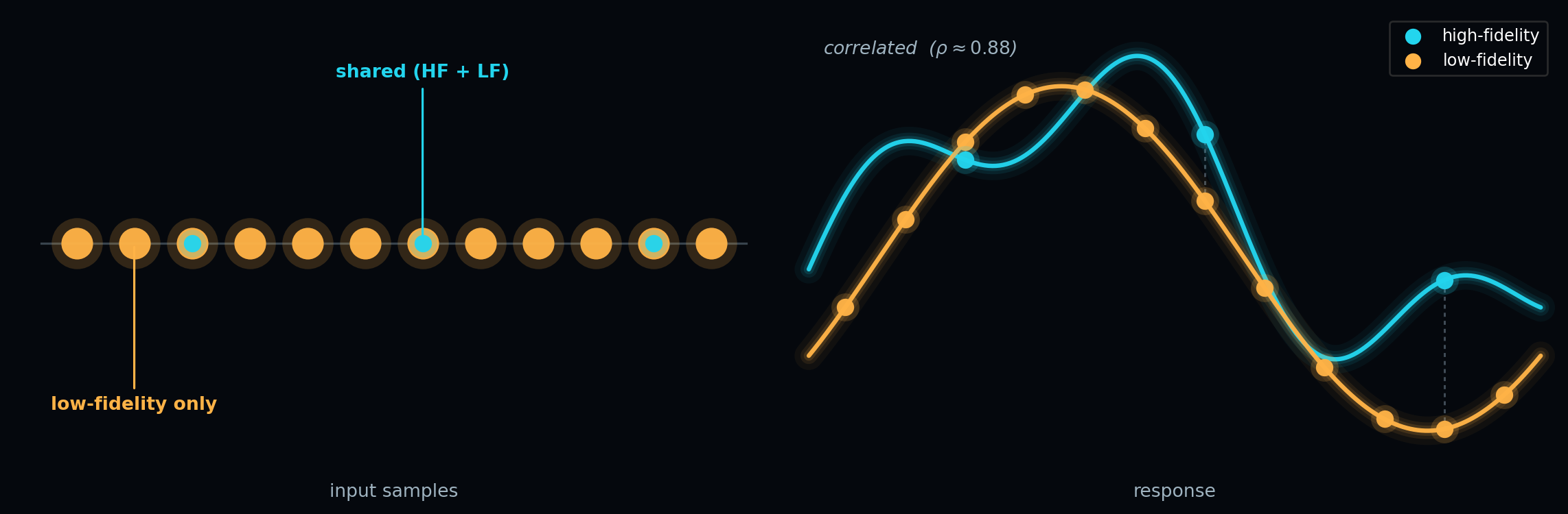
Figure 2 illustrates the two sample sets. Unlike CVMC, where every sample is evaluated by both models, ACV uses a small set of shared samples (where both models are evaluated) plus a larger set of LF-only samples (where only the cheap model is evaluated). The shared samples provide the correlated correction; the LF-only samples sharpen the estimate of \(\mu_\kappa\).
The Allocation Problem
The total cost of one ACV estimate is
\[ P = N\,(c_\alpha + r\, c_\kappa), \tag{2}\]
where \(c_\alpha\) and \(c_\kappa\) are the per-sample costs of the two models. The extra \(r\, c_\kappa\) per HF sample buys a more accurate estimate of \(\mu_\kappa\), which tightens the correction.
As in CVMC, the goal is to minimize estimator variance subject to the budget:
\[ \min_{N,\, r,\, \eta} \;\mathbb{V}[\hat{\mu}_\alpha^{\text{ACV}}] \quad \text{subject to} \quad N\,(c_\alpha + r\, c_\kappa) \leq P. \tag{3}\]
The weight \(\eta\) decouples from the allocation: its optimum depends on the model covariance and \(r\) but not on \(N\) (see ACV Analysis). After plugging in \(\eta^*\), the variance is \(\sigma^2_\alpha\, \gamma(r) / N\) where \(\gamma(r) = 1 - \frac{r-1}{r}\rho^2\) is the reduction factor below. The budget constraint gives \(N = P / (c_\alpha + r\, c_\kappa)\), so for the two-model case the problem reduces to a one-dimensional optimization over \(r\):
\[ \min_{r \geq 1} \;\frac{\sigma^2_\alpha}{P}\; (c_\alpha + r\, c_\kappa)\; \left(1 - \frac{r - 1}{r}\,\rho^2\right). \]
This has a closed-form solution (derived in the analysis tutorial). The key point is that unlike CVMC — where the allocation is trivially determined by the budget — ACV introduces a genuine trade-off: spending more on LF samples (larger \(r\)) tightens the correction but leaves fewer resources for HF samples (smaller \(N\)). The optimal \(r^*\) balances these two effects.
With many LF models, there is one ratio \(r_\alpha\) per LF model and the allocation becomes a multi-dimensional constrained optimization. With group ACV, the free parameters are the sample counts of every partition and the problem is high-dimensional. The closed-form solution is unique to the two-model case.
Variance Reduction Depends on \(r\)
With the optimal \(\eta\) (derived in ACV Analysis), the variance reduction factor is
\[ \gamma = 1 - \frac{r - 1}{r}\,\rho^2_{\alpha\kappa}. \tag{4}\]
Two limits are instructive. As \(r \to 1^+\) (almost no extra LF samples), \(\gamma \to 1\) and ACV offers no improvement over plain MC. As \(r \to \infty\) (very many LF samples), \(\gamma \to 1 - \rho^2_{\alpha\kappa}\), recovering the full CVMC variance reduction. For finite \(r\), ACV lies strictly between these bounds.
Figure 3 shows how rapidly \(\gamma\) approaches the CVMC limit. Even modest \(r\) (e.g. \(r = 10\)) recovers \(90\%\) of the maximum variance reduction. Because \(f_\kappa\) is cheap, large \(r\) is usually affordable.

Key Takeaways
- CVMC requires \(\mu_\kappa\) to be known exactly; in practice it is not, which motivates ACV
- Estimating \(\mu_\kappa\) from the same HF samples gives zero correction; a separate LF sample set is needed
- The ACV estimator uses \(\mathcal{Z}_N\) (shared) and \(\mathcal{Z}_{rN} \supset \mathcal{Z}_N\) (LF only); it is unbiased for any \(r > 1\)
- Variance reduction is \(1 - \frac{r-1}{r}\rho^2\), interpolating between no reduction (\(r \to 1\)) and full CVMC reduction (\(r \to \infty\))
- Because LF evaluations are cheap, large \(r\) is usually affordable
Exercises
Figure 1 shows that a noisy correction still reduces variance compared to plain MC. Is this always true, or can a bad \(\mu_\kappa\) estimate make things worse?
From Equation 4, find the value of \(r\) at which ACV achieves \(95\%\) of the CVMC variance reduction for \(\rho = 0.9\). How does your answer change for \(\rho = 0.5\)?
Suppose \(C_\kappa = 0.01 C_\alpha\) (LF is 100× cheaper). For a fixed total budget equal to \(N C_\alpha\), roughly how large can you make \(r\)? What variance reduction does this buy for \(\rho = 0.9\)?
Next Steps
- ACV Analysis — Derive \(\gamma = 1 - \frac{r-1}{r}\rho^2\), the optimal \(\eta\), and the optimal \(r\) for a fixed budget
- API Cookbook — Use the PyApprox ACV API end-to-end
- General ACV — Extend ACV to many low-fidelity models
Tip
Ready to try this? See API Cookbook → Universal Workflow.
References
- [GGEJJCP2020] A. Gorodetsky, S. Geraci, M. Eldred, J. Jakeman. A generalized approximate control variate framework for multifidelity uncertainty quantification. Journal of Computational Physics, 408:109257, 2020. DOI