---
title: "Group ACV: Solving the Allocation Problem"
subtitle: "PyApprox Tutorial Library"
description: "How to drive the sample-allocation optimizer for group ACV estimators. The default recipe is SLSQP with log-space variable scaling. The MLBLUE convex SDP reformulation, although mathematically appealing, is unreliable with the cvxpy default backends (CLARABEL, SCS) on realistic multifidelity problems due to a Schur-complement conditioning gap; SLSQP remains the workhorse. Mean-guided pruning rescues variance estimation at tight budgets."
tutorial_type: usage
topic: multi_fidelity
difficulty: intermediate
estimated_time: 17
render_time: 100
prerequisites:
- group_acv_concept
- group_acv_multistat_concept
tags:
- multi-fidelity
- group-acv
- optimization
- slsqp
- mean-guided
format:
html:
code-fold: false
code-tools: true
toc: true
execute:
echo: true
warning: false
jupyter: python3
---
::: {.callout-tip collapse="true"}
## Download Notebook
[Download as Jupyter Notebook](notebooks/group_acv_optimization.ipynb)
:::
## Learning Objectives
After completing this tutorial, you will be able to:
- Configure `GroupACVAllocationOptimizer` with the default `AllocationProblemConfig`
and explain why log-space variable scaling and inequality budget form are the
recommended defaults
- Recognize the failure signatures of alternative scaling configurations: gentle
widening of the optimality gap for `none`/`constraint_only`, and catastrophic
non-monotonic convergence for `full`
- Understand why `MLBLUESPDAllocationOptimizer`, despite solving a convex
reformulation, can produce much worse allocations than SLSQP on problems
with many subsets when using the cvxpy default backends (CLARABEL, SCS)
- Diagnose why direct SLSQP fails for variance estimation at tight budgets — the
$n \geq 2$ dead-region constraint — and use `MeanGuidedSubsetFitter` to recover
## Prerequisites
Complete [Group ACV Concept](group_acv_concept.qmd) for the framework and
[Group ACV Multi-Statistic Concept](group_acv_multistat_concept.qmd) for the
variance-estimation pieces. The earlier tutorials introduced
`GroupACVEstimatorIS`, `MLBLUEEstimator`, and `MeanGuidedSubsetFitter` without
discussing how their allocators are configured; this tutorial fills that gap.
## Quick Recap of the Optimization Problem
The group ACV allocator minimizes the predicted estimator variance
$(\mathbf{e}^0)^\top (R\, C^{-1} R^\top)^{-1} \mathbf{e}^0$ over partition sample
counts $\{m^k\}_{k=1}^K$, subject to a budget constraint
$\sum_k m^k c^k \leq P$ and lower bounds on each $m^k$. The lower bound
$\mathrm{lb}_k$ is the **continuous dead threshold** of the target statistic — zero
for mean estimation (a partition can vanish), two for variance estimation (an
unbiased sample variance needs $n \geq 2$ observations).
The full derivation lives in
[Group ACV Analysis §11](group_acv_analysis.qmd#sec-connection-allocation). This
tutorial focuses on the practical question: which optimizer settings make the
solver actually find a good allocation, and how do you handle the cases where
the defaults fail?
## Setup
```{python}
import numpy as np
import matplotlib.pyplot as plt

from pyapprox.util.backends.numpy import NumpyBkd
from pyapprox_benchmarks.statest import PolynomialEnsembleBenchmark
from pyapprox.statest.statistics import MultiOutputMean, MultiOutputVariance
from pyapprox.statest.groupacv import (
    GroupACVAllocationOptimizer,
    GroupACVEstimatorIS,
    MeanGuidedSubsetFitter,
    MLBLUEEstimator,
    MLBLUESPDAllocationOptimizer,
    get_model_subsets,
)
from pyapprox.statest.groupacv.variable_space import AllocationProblemConfig
from pyapprox.optimization.minimize.scipy.slsqp import ScipySLSQPOptimizer

bkd = NumpyBkd()
benchmark = PolynomialEnsembleBenchmark(bkd, nmodels=5)
costs = benchmark.problem().costs()
cov = benchmark.ensemble_covariance()
nmodels = 5
subsets = get_model_subsets(nmodels, bkd)
print(f"{nmodels} models, {len(subsets)} candidate subsets")
```
Throughout this tutorial, pilot quantities ($\boldsymbol{\Sigma}$, $W$, $B$ —
defined in [Group ACV Multi-Statistic Concept](group_acv_multistat_concept.qmd))
are computed via exact Gauss quadrature on the known polynomial model functions,
eliminating pilot sampling noise so that optimizer behavior is isolated from
pilot estimation effects.
## The Default Recipe: SLSQP + log/inequality
For any group ACV problem with mean, variance, or mean+variance target, the
default optimizer recipe is **SLSQP** as the local solver, with
`variable_scaling="log"` and `budget_constraint_form="inequality"` on the
allocation problem config.
```{python}
stat_mean = MultiOutputMean(1, bkd)
stat_mean.set_pilot_quantities(cov)

template = GroupACVEstimatorIS(stat_mean, costs, model_subsets=subsets)
log_ineq = AllocationProblemConfig(
    variable_scaling="log",
    budget_constraint_form="inequality",
)
allocator = GroupACVAllocationOptimizer(
    template,
    optimizer=ScipySLSQPOptimizer(maxiter=1000, ftol=1e-6),
    problem_config=log_ineq,
)
result = allocator.optimize(target_cost=500.0, round_nsamples=False)
cov_est = template._covariance_from_npartition_samples(
    result.npartition_samples
)
print(f"success    = {result.success}")
print(f"actual cost = {result.actual_cost:.2f}")
print(f"variance   = {float(bkd.to_numpy(cov_est[0,0])):.3e}")
```
Three knobs determine the recipe and matter in this order:
- **Variable scaling.** The optimizer works in a transformed variable space
$m_k = g(n_k)$. For `"log"`, $m_k = \log n_k$. The transformation equalizes
the dynamic range of partition sample counts when model costs span many
orders of magnitude — without it the gradient with respect to the cheap-model
partitions is many orders of magnitude smaller than the gradient with respect
to the HF partition, and SLSQP terminates prematurely.
- **Budget constraint form.** `"inequality"` is the default. Some optimizers
may perform better with `"equality"`, but SLSQP produces the same result
with either form on this benchmark.
- **Lower bound on $m_k$.** Automatically set from the statistic's dead
threshold: zero for mean estimation, two for variance. Users should not
need to override this.
## Choosing the Objective: Trace vs Log-Determinant
`GroupACVAllocationOptimizer` defaults to `GroupACVLogDetObjective` — it
minimizes $\log\det(\mathrm{Cov})$ of the estimator covariance, not
$\mathrm{tr}(\mathrm{Cov})$. Most users never notice this default because
for single-QoI problems (`nqoi = 1`) the covariance is a $1 \times 1$ matrix
and both objectives reduce to minimizing the same scalar variance — the
logarithm in log-det is a monotone transform that does not change the
optimum.
For multi-QoI estimation the two objectives are genuinely different. The
trace is the sum of marginal QoI variances, so trace-optimal allocations
minimize the *average* uncertainty across QoIs. The log-determinant is the
logarithm of the volume of the joint confidence ellipsoid, so log-det-optimal
allocations minimize the *joint* uncertainty. The two objectives put their
budget on different partitions whenever the QoIs have different correlation
structures across the model ensemble.
Swap objectives via the `objective` argument:
```{python}
from pyapprox.statest.groupacv import (
    GroupACVLogDetObjective,
    GroupACVTraceObjective,
)

allocator_trace = GroupACVAllocationOptimizer(
    template,
    optimizer=ScipySLSQPOptimizer(maxiter=1000, ftol=1e-6),
    problem_config=log_ineq,
    objective=GroupACVTraceObjective(),  # default is GroupACVLogDetObjective
)
```
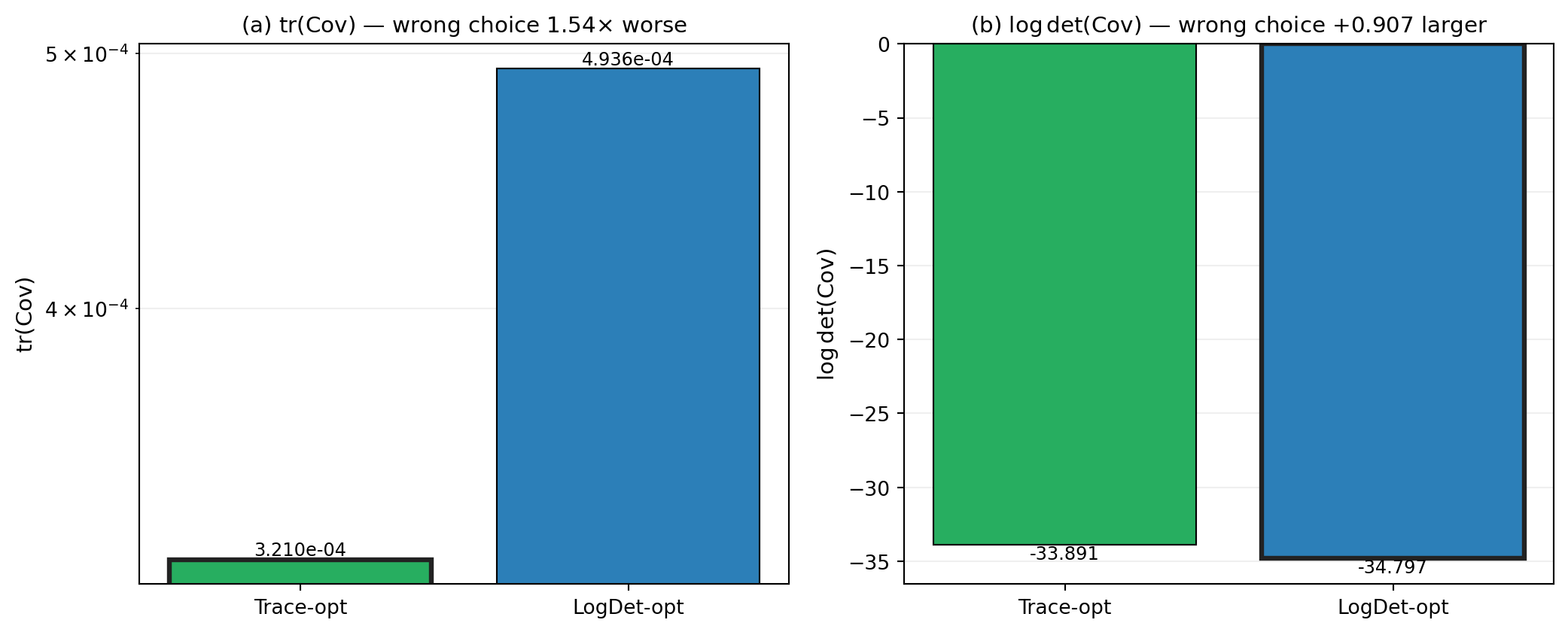
@fig-trace-vs-logdet runs both objectives on the multi-output ensemble
benchmark (3 models, 3 QoIs) and reports the trace and log-det of the
resulting estimator covariance for each. The trace-optimal allocation wins
on the trace metric; the log-det-optimal allocation wins on the log-det
metric. The cross-evaluations quantify the penalty for using the wrong
objective.
```{python}
#| echo: false
#| fig-cap: "Cross-evaluation of trace-optimal and log-det-optimal allocations on the 3-model 3-QoI multi-output benchmark at $P = 100$. **(a)** Trace of the estimator covariance. The trace-optimal allocation (green) achieves the smallest trace; the log-det-optimal allocation (blue) is larger by the factor in the title. **(b)** Log-determinant. The log-det-optimal allocation wins; the trace-optimal allocation has a larger log-det by the additive offset in the title. The bar with the heavy black outline is the winner of each panel."
#| label: fig-trace-vs-logdet
from pyapprox_tutorials.figures._group_acv_optimization import (
plot_trace_vs_logdet,
)
fig, axes = plt.subplots(1, 2, figsize=(11, 4.5))
plot_trace_vs_logdet(axes)
plt.tight_layout()
plt.show()
```
Two practical points come out of this:
- For single-QoI problems the choice is invisible — keep the default.
- For multi-QoI problems, pick the objective that matches the downstream
decision. If users will report each QoI's uncertainty separately, trace
is the natural target. If users will form joint confidence regions or
compare estimators by total information content, log-det is the natural
target. The PyApprox default of log-det matches the multi-output ACV
literature convention; choose trace when your downstream consumers think
in marginal-variance terms.
## Why Log-Space Matters: How the Alternatives Fail
`AllocationProblemConfig.variable_scaling` accepts four values: `"none"`,
`"constraint_only"`, `"full"`, and `"log"`. The other three exist for diagnostic
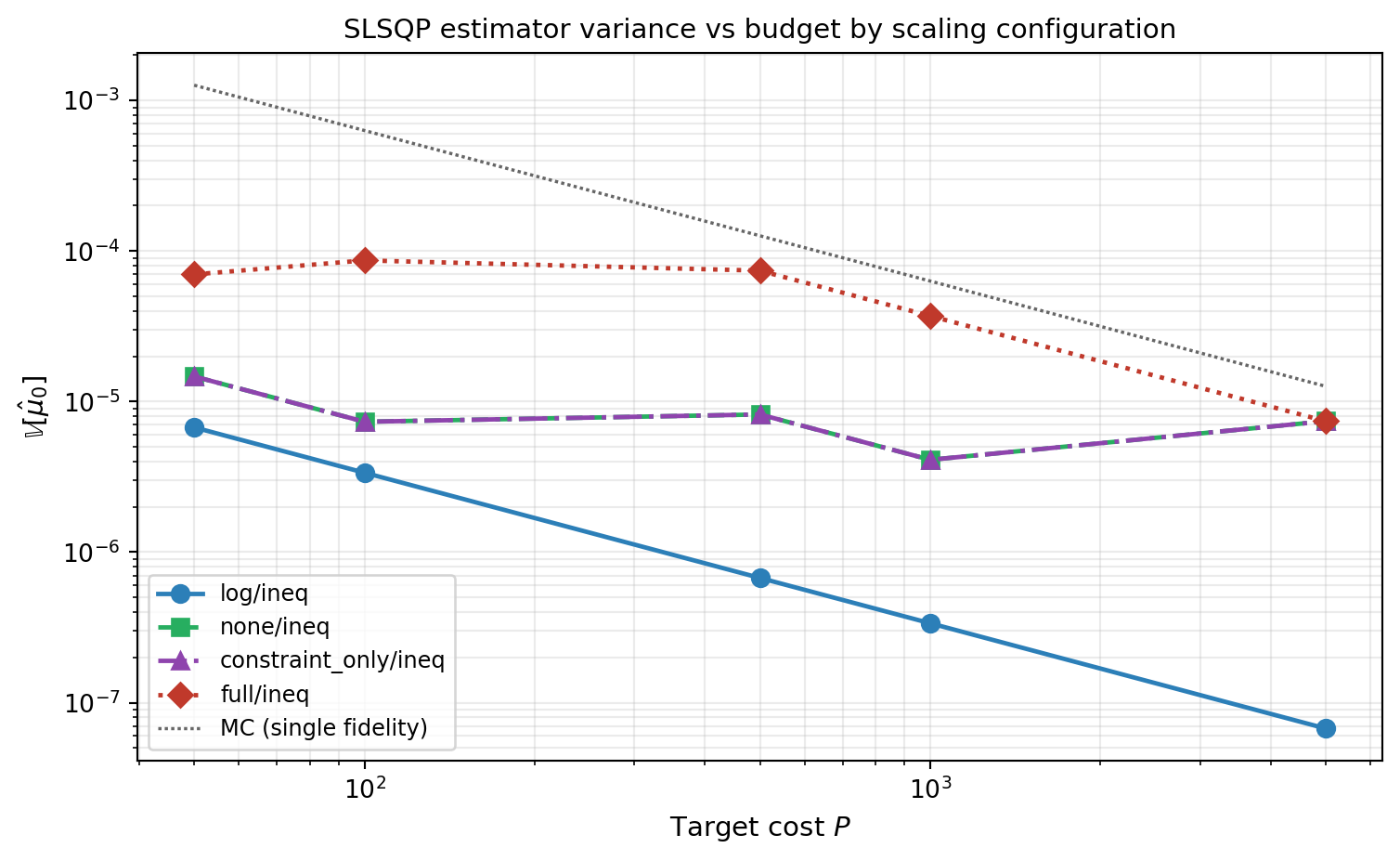
and special-case use. @fig-scaling-comparison contrasts SLSQP's behavior with
each, sweeping the target budget on the five-model polynomial benchmark for
mean estimation.
```{python}
#| echo: false
#| fig-cap: "Estimator variance vs budget for SLSQP with four scaling configurations, all using inequality budget form. **log/ineq** (blue, solid) is monotonic and consistently best. **none/ineq** (green, dashed) and **constraint_only/ineq** (purple, dot-dashed) are competitive at small to moderate budgets but their gap to log/ineq widens as the budget grows. **full/ineq** (red, dotted) exhibits non-monotonic convergence: the variance at budget=1000 is worse than at budget=500, and at budget=5000 the optimizer terminates after only ~23 iterations stuck near the initial guess — a clear gradient-pathology signature. The dotted gray reference is single-fidelity Monte Carlo at the same budget."
#| label: fig-scaling-comparison
from pyapprox_tutorials.figures._group_acv_optimization import (
plot_scaling_comparison,
)
fig, ax = plt.subplots(figsize=(8, 5))
plot_scaling_comparison(ax)
plt.tight_layout()
plt.show()
```
Three patterns are worth committing to memory:
**Full scaling is worse with more budget.** The `full` configuration rescales
$m_k = (c_k / c_{\min}) n_k$, so partitions involving expensive models live on
a much larger scale than partitions on cheap models. As the budget grows the
optimum allocation shifts mass onto cheap LF models, which sharpens the cost
ratio in the variables, which worsens the conditioning, which causes SLSQP to
stop earlier with a poorer iterate. The non-monotonic variance curve is the
visible signature.
**None and constraint-only scaling degrade slowly.** Both work in raw $n$-space
and differ only in whether the constraint output is normalized. They produce
nearly identical iterates at moderate budgets but lose roughly a factor of two
in variance relative to log scaling by budget = 5000. The optimizer is not
stuck; the local minimum it finds is just slightly worse than log scaling's.
**Log scaling is the workhorse.** Across more than three orders of magnitude
in budget, log scaling is consistently the best of the four. There is no
budget regime in this benchmark where another scaling beats it. Use it as the
default unless you have a specific reason to deviate.
## The MLBLUE Mean-Only Convex Formulation: Theory and a Numerical Trap
When the target statistic is the mean and the group structure uses independent
samples across subsets, the allocation problem is **convex** and admits a
semidefinite-programming (SDP) reformulation. The SDP form was introduced by
[CWARXIV2023] precisely to fix a numerical issue in the original
[SUSIAMUQ2020] formulation: when models are discarded, $\Psi(\mathbf{m})$
becomes singular and Schaden-Ullmann had to add a shift $\Psi_\delta = \Psi +
\delta I$ with a $\delta$ that is delicate to tune. The CWW SDP reformulation
avoids this by using the Moore-Penrose pseudoinverse and the PSD constraint,
and they report that CVXOPT's `conelp` solver converges reliably on their PDE
benchmarks where IPOPT and SciPy's `trust-constr` either need careful tuning
or fail outright. In theory the SDP returns the global optimum.
In practice, the SDP form also has a conditioning issue — *a different one*
from the singularity that motivated it — that makes the cvxpy-default backends
(CLARABEL, SCS) unreliable on realistic multifidelity problems. Before
showing it, here is the API for completeness:
```{python}
mlblue = MLBLUEEstimator(stat_mean, costs, model_subsets=subsets)
spd_allocator = MLBLUESPDAllocationOptimizer(mlblue)
spd_result = spd_allocator.optimize(target_cost=500.0, round_nsamples=False)
spd_cov_est = mlblue._covariance_from_npartition_samples(
    spd_result.npartition_samples
)
print(f"SPD success = {spd_result.success}")
print(f"SPD variance = {float(bkd.to_numpy(spd_cov_est[0,0])):.3e}")
```
The SDP encodes the variance-minimization problem via a Schur complement: a
scalar variable $t$ is constrained to satisfy
$$
\begin{bmatrix}
\Psi(\mathbf{m}) & A^{\!\top} \\
A & t
\end{bmatrix}
\succeq 0
\quad\iff\quad
t \;\geq\; A\,\Psi(\mathbf{m})^{-1} A^{\!\top},
$$
and the SDP minimizes $t$. Mathematically this is equivalent to minimizing the
estimator variance.
Numerically the encoding suffers a scale gap. The diagonal entries of $\Psi$
grow with the partition sample counts, which themselves grow with the budget
— at $P = 500$ on the five-model polynomial benchmark the optimal allocation
has $\max_k m^k \approx 2.3 \times 10^5$, and $\Psi$ entries reach $\sim 10^6$.
The optimal $t$ is the estimator variance, $\sim 4 \times 10^{-6}$. The ratio
$$
\kappa_{\text{SDP}} \;\equiv\; \frac{\max(\Psi)}{t} \;\sim\; 10^{11}
$$
is the condition number of the Schur-complement block matrix. The SDP solvers
shipped with cvxpy — specifically **CLARABEL** (the cvxpy default) and
**SCS** — drive the duality gap toward zero by following the central path of
the barrier-regularized problem, but the central-path Newton system inherits
this conditioning. When $\kappa_{\text{SDP}}$ exceeds roughly $10^8$ — which
it does for any realistic MLBLUE problem with more than a couple of subsets
— the solver's enforcement of the PSD constraint loses accuracy in proportion
to the conditioning, and the returned $t$ sits above the true Schur complement
bound. The duality gap report (typically $10^{-12}$ or smaller) tells you the
*internal* equilibrated KKT residual is tight; it does not tell you the
primal variable $t$ is close to its true minimum. CVXOPT — the solver CWW
used successfully on their PDE benchmarks — has different numerical machinery
and may avoid this failure mode; we have not tested it on the polynomial
benchmark used here.
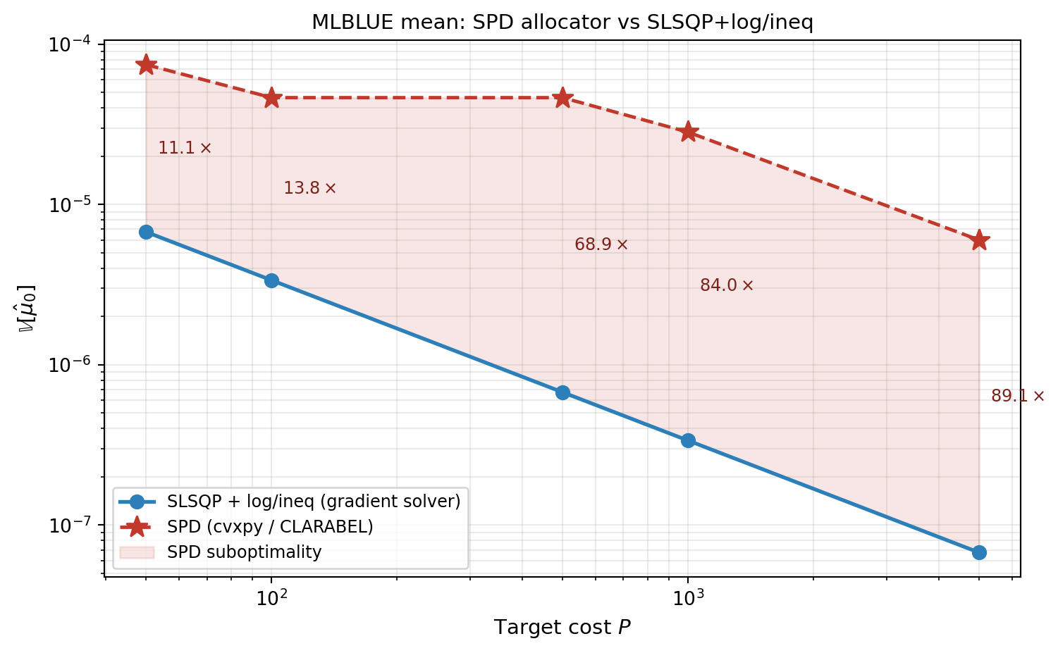
Concretely on this benchmark: at $P = 500$, the SDP returns $t = 1.3 \times
10^{-5}$ but the variance at the SDP's own allocation is $7.1 \times 10^{-6}$
— the SDP is **already 1.8× suboptimal at its own returned point**, and the
SLSQP allocation is a further $1.7\times$ better. The gap to SLSQP is
present **at every budget shown** in @fig-spd-vs-slsqp, including the
smallest — SPD is roughly $2.5\times$ worse than SLSQP at $P = 10$ already
— and grows past $50\times$ by $P = 5000$. Tightening solver tolerances does
not help: we tested CLARABEL with `eps_abs/rel/infeas = 1e-12` and SCS with
`eps_abs/rel = 1e-12, max_iters = 100000`, and both solvers converge cleanly
to the same suboptimal allocation as their defaults.
@fig-spd-vs-slsqp shows the gap across the budget sweep — SPD is
substantially worse than SLSQP at every budget tested, with the
magnitude of the gap growing as the optimal allocation's dynamic
range grows.
```{python}
#| echo: false
#| fig-cap: "MLBLUE mean estimation: variance achieved by the SPD allocator (red, dashed, stars) vs SLSQP+log/ineq (blue, solid, circles) across budgets on the five-model polynomial benchmark. SPD here is solved via cvxpy with the CLARABEL backend (the cvxpy default). SPD is substantially worse than SLSQP at every budget shown — the gap is already a factor of a few at $P = 50$ and grows to roughly $50\\times$ by $P = 5000$. The shaded region is the SPD suboptimality, with ratio annotations at each point where the gap exceeds $1.2\\times$. The widening with budget reflects growing Schur-complement conditioning $\\kappa_{\\text{SDP}}$, not numerical tolerance: both CLARABEL and SCS converge cleanly with duality gap below $10^{-12}$ to the suboptimal point. SPD agrees with SLSQP only when the subset count is small enough that $\\Psi$ stays low-dimensional (verified separately on a two-subset version of this problem)."
#| label: fig-spd-vs-slsqp
from pyapprox_tutorials.figures._group_acv_optimization import (
plot_spd_vs_slsqp,
)
fig, ax = plt.subplots(figsize=(8, 5))
plot_spd_vs_slsqp(ax)
plt.tight_layout()
plt.show()
```
::: {.callout-warning}
## SPD as a workhorse: not recommended with cvxpy default solvers
`MLBLUESPDAllocationOptimizer` is **not recommended as the default allocator
for MLBLUE mean estimation** when using the cvxpy default backend (CLARABEL)
or SCS. SLSQP with `log/ineq` configuration on `GroupACVEstimatorIS` (or
equivalently on `MLBLUEEstimator`, which inherits the same covariance
machinery) returns a strictly better allocation in every regime we tested
on the polynomial five-model benchmark.
:::
The SPD allocator is preserved in PyApprox for two reasons. First, on very
small problems with **only two or three subsets** — where $\Psi$ stays
low-dimensional and $\kappa_{\text{SDP}}$ stays well below $10^7$ across
all budgets — even CLARABEL agrees with SLSQP to high precision and provides
a useful sanity check on the gradient solver. (We have confirmed exact
agreement between SPD and SLSQP across the full budget sweep on a literal
two-subset version of this benchmark.) Second, even when the SDP result is
suboptimal, it is typically in the right *basin* of the convex landscape —
passing `init_guess=spd_result.npartition_samples` to
`GroupACVAllocationOptimizer.optimize()` is a sensible warm-start that
places SLSQP near the optimum (exercise 3).
## Variance Estimation and the $n \geq 2$ Dead Region
The sample variance $\hat{\sigma}^2 = \frac{1}{m-1}\sum_i (f^{(i)} - \bar{f})^2$
requires at least two samples to be defined and unbiased. The per-partition
covariance block $C^k$ for variance estimation contains factors $1/(m^k - 1)$
that diverge at $m^k = 1$ and become negative for non-integer $m^k \in (0, 1)$.
PyApprox encodes this via `MultiOutputVariance.continuous_dead_threshold = 2`,
and the allocation optimizer enforces $m^k \geq 2$ for every partition by
default.
This bound has a consequence at tight budgets. With $K = 2^M - 1$ candidate
subsets, the minimum feasible cost is roughly $2 \sum_k c^k$, which can exceed
modest target budgets. Even when feasible, allocating two samples to every
uninformative partition wastes the budget that should go to the few partitions
actually carrying signal.
A direct SLSQP solve on `GroupACVEstimatorIS` with `MultiOutputVariance` at
small budgets either fails outright or returns a poor local minimum. The
fix is **mean preprocessing**.
## Mean-Guided Preprocessing for Variance Estimation
The key observation: the same group structure that is optimal for variance
estimation tends to be approximately optimal for mean estimation on the same
problem, and the mean problem has zero dead threshold so partitions can drop
to zero freely. `MeanGuidedSubsetFitter` exploits this in two stages.
**Stage 1 — screening.** Build a copy of the estimator with a `MultiOutputMean`
statistic that shares the target stat's covariance. Solve the mean allocation
with `bounds_lb=1e-8` so partitions can shrink to ~0. The partitions with
post-solve sample counts above `activity_threshold` (default 1.0) are the
**active** set; the rest are pruned.
**Stage 2 — reduced target solve.** Construct a new estimator restricted to the
active subsets only, then run the target-statistic (variance, mean+variance)
optimization on this much smaller problem.
```{python}
stat_var = MultiOutputVariance(1, bkd)
cov_var = benchmark.covariance_matrix()
W_var = benchmark.covariance_of_centered_values_kronecker_product()
stat_var.set_pilot_quantities(cov_var, W_var)

fitter = MeanGuidedSubsetFitter(
    stat_var, costs, GroupACVEstimatorIS,
    candidate_subsets=subsets,
    optimizer=ScipySLSQPOptimizer(maxiter=1000, ftol=1e-6),
    problem_config=log_ineq,
)
guided = fitter.fit(target_cost=50.0, min_nhf_samples=1)
print(f"pruned {guided.partitions_pruned()} of {len(subsets)} partitions")
print(f"active subset indices: {guided.active_subset_indices}")
var_est = float(bkd.to_numpy(guided.best_estimator.covariance()[0, 0]))
print(f"variance estimator var = {var_est:.3e}")
```
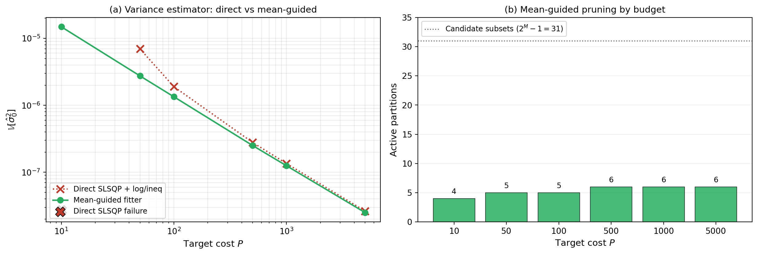
@fig-variance-rescue compares direct SLSQP against the mean-guided fitter
across budgets, and shows how aggressively the fitter prunes.
```{python}
#| echo: false
#| fig-cap: "**(a)** Variance-estimator variance vs budget. Direct SLSQP+log/ineq (red, dotted) fails at small budgets (X markers on the budget axis mark failures) and underperforms even where it succeeds. The mean-guided fitter (green, solid) returns a feasible allocation at every budget shown and finds a lower variance at each. **(b)** Active partitions retained after Stage 1 screening. The benchmark has $2^M - 1 = 31$ candidate subsets (gray dashed line). At tight budgets the fitter keeps only a handful — the few that contribute signal — and lets the budget go where it matters."
#| label: fig-variance-rescue
from pyapprox_tutorials.figures._group_acv_optimization import (
plot_variance_rescue,
)
fig, axes = plt.subplots(1, 2, figsize=(13, 4.5))
plot_variance_rescue(axes)
plt.tight_layout()
plt.show()
```
Two operational consequences:
- For variance estimation, treat `MeanGuidedSubsetFitter` as the default
pathway, not as an escape hatch for failure cases. Even when direct SLSQP
succeeds, the fitter usually finds a better allocation because the reduced
problem is easier to optimize.
- The Stage-1 mean solve is the same order of cost as the Stage-2 variance
solve, and both are small relative to the cost of generating simulation data.
::: {.callout-note}
## Mean-guided pruning is distinct from "allocate for mean, evaluate variance"
The fitter uses the mean only to *identify* active partitions; the Stage-2
allocation is then re-optimized for the variance target. It does not
reuse the mean's *sample counts* for variance estimation. A related but
different question — what suboptimality you incur by allocating samples
for mean estimation and then computing variance (or mean+variance) from
those same samples — is a problem-formulation question rather than an
optimizer-tactics question. See [Group ACV Multi-Statistic
Concept](group_acv_multistat_concept.qmd) for the joint vs standalone
discussion that frames that trade-off.
:::
## Practical Recipe
The following table summarizes the allocator choice for common configurations.
| Scenario | Allocator |
|---------------------------------------------------|---------------------------------------------------------------------------|
| Mean estimation, any group structure | `GroupACVAllocationOptimizer` + SLSQP + `log/ineq` |
| MLBLUE mean (independent subsets) | Same as above; `MLBLUEEstimator` inherits the covariance machinery |
| Variance or mean+variance estimation | `MeanGuidedSubsetFitter` + SLSQP + `log/ineq` |
| Multi-QoI, marginal variances matter most | Add `objective=GroupACVTraceObjective()` to any of the above |
| Multi-QoI, joint uncertainty matters most | Keep the default `GroupACVLogDetObjective` |
| Want to try SDP on a problem with few subsets | `MLBLUESPDAllocationOptimizer` (default CLARABEL); for more reliability, pass `solver_name="CVXOPT"` |
| Want a coarse SDP-based initial guess for SLSQP | `MLBLUESPDAllocationOptimizer` → pass `result.npartition_samples` as `init_guess` to `GroupACVAllocationOptimizer.optimize()` |
| Allocator fails despite reasonable setup | Increase `maxiter` / tighten `ftol`; if still failing, file a bug report |
A few rules that hold across all scenarios: always use `log/ineq` as the
problem config unless you have a specific reason to deviate, always pass an
explicit `ScipySLSQPOptimizer` rather than relying on the default optimizer,
and check `result.success` before consuming `result.npartition_samples`.
## Key Takeaways
- The default optimizer recipe for group ACV is SLSQP with
`AllocationProblemConfig(variable_scaling="log", budget_constraint_form="inequality")`.
- The default objective is `GroupACVLogDetObjective`. For single-QoI
problems this is equivalent to minimizing the scalar variance. For
multi-QoI, trace-optimal and log-det-optimal allocations differ
(see @fig-trace-vs-logdet) — pick the objective that matches the downstream
decision.
- Other variable scalings degrade at high budgets: `none` and `constraint_only`
widen their gap to log-space gradually; `full` exhibits non-monotonic
convergence and is essentially never the right choice (see @fig-scaling-comparison).
- For mean estimation with MLBLUE-style independent subsets, the allocation
problem is convex in theory — but the SDP reformulation
(`MLBLUESPDAllocationOptimizer`) with the cvxpy default backends
(CLARABEL, SCS) suffers a Schur-complement conditioning gap between the
$\Psi$ block and the variance scalar $t$, leading to allocations that are
2–50× worse than SLSQP on the polynomial five-model benchmark (see
@fig-spd-vs-slsqp). Use SLSQP with `log/ineq` for MLBLUE mean estimation
as the workhorse; treat the SDP allocator as a coarse initialization or a
small-subset sanity check.
- Variance estimation enforces $m^k \geq 2$ per partition, which makes direct
SLSQP fail or waste budget at tight budgets. `MeanGuidedSubsetFitter`
screens with a cheap mean solve to find the active subset, then runs the
variance optimization on the reduced estimator (see @fig-variance-rescue).
## Exercises
1. Rerun the SLSQP scaling comparison with `budget_constraint_form="equality"`
instead of `"inequality"`. Does the failure pattern of `full` scaling
change? Why might equality form be slightly harder for an active-set
solver like SLSQP near the optimum?
2. Take a budget where direct SLSQP succeeds on the variance problem (say
$P = 1000$). Run both the direct allocator and `MeanGuidedSubsetFitter`.
Confirm the fitter finds an equal-or-better allocation. *(Hint: read off
`guided.active_subset_indices` and compare to the partitions with non-zero
counts in the direct result.)*
3. Run `MLBLUESPDAllocationOptimizer` and SLSQP+log/ineq on the MLBLUE mean
problem at $P = 100$ and $P = 5000$. Compute the ratio of SDP variance to
SLSQP variance at each budget. Verify that the ratio grows with budget,
and explain in terms of the conditioning number $\kappa_{\text{SDP}}$.
Then warm-start SLSQP from the SPD allocation (pass `init_guess`) and
verify it recovers the SLSQP-from-default-init result in a small number
of iterations.
4. The `MeanGuidedSubsetFitter` has an `activity_threshold` parameter
(default $1.0$). Predict what happens if you set it to $10^{-1}$ on
the variance problem at $P = 5000$. Verify your prediction.
5. Run the multi-QoI demo in @fig-trace-vs-logdet at $P = 1000$ instead of
$P = 100$. Does the ratio of trace-at-logdet-opt to trace-at-trace-opt
shrink or grow with budget? Reason about why.
6. For a single-QoI version of the polynomial benchmark, solve with
`GroupACVTraceObjective` and `GroupACVLogDetObjective` at the same budget.
Verify numerically that the resulting allocations agree (up to optimizer
tolerance) and explain in one sentence why.
## Next Steps
- [Group ACV Mixed Concept](group_acv_mixed_concept.qmd) — combine known
statistics with mean-guided preprocessing for variance estimation
- [API Cookbook](multifidelity_estimation_cookbook.qmd#estimator-quick-reference)
— runnable end-to-end recipes for every group ACV estimator
- [Pilot Studies Concept](pilot_studies_concept.qmd) — how the pilot study
size interacts with optimizer choice at small budgets
## References
- [GJE2024] A. Gorodetsky, J. Jakeman, M. Eldred. *Grouped approximate control
variate estimators.* arXiv:2402.14736, 2024.
[DOI](https://doi.org/10.48550/arXiv.2402.14736)
- [SUSIAMUQ2020] D. Schaden, E. Ullmann. *On multilevel best linear unbiased
estimators.* SIAM/ASA J. Uncertainty Quantification 8(2):601–635, 2020.
[DOI](https://doi.org/10.1137/19M1263534)
- [CWARXIV2023] M. Croci, K. Willcox, S. Wright. *Multi-output multilevel best
linear unbiased estimators via semidefinite programming.* Computer Methods
in Applied Mechanics and Engineering, 2023.
[DOI](https://doi.org/10.1016/j.cma.2023.116130)
- [Kraft1988] D. Kraft. *A software package for sequential quadratic programming.*
DFVLR Forschungsbericht DFVLR-FB 88-28, 1988. (The SLSQP algorithm used by
SciPy and PyApprox.)