Learning from Experiments: Bayesian Optimal Experimental Design
PyApprox Tutorial Library
What Expected Information Gain measures and why it is the right objective for choosing experiments.
TipDownload Notebook
Learning Objectives
After completing this tutorial, you will be able to:
- Explain what Expected Information Gain (EIG) measures in terms of KL divergence
- Distinguish EIG-based (parameter-focused) OED from goal-oriented OED
- Describe qualitatively why the double-loop Monte Carlo approximation is needed
- Identify the tradeoff between inner and outer sample budgets
Prerequisites
Complete Not All Experiments Are Equal before this tutorial.
From Posterior Covariance to Information Gain
In the introductory tutorial we compared experimental designs by looking at the posterior covariance determinant. That works for linear Gaussian problems, but it conceals an important question: how do we measure “how much we learned” in a way that averages over all possible experimental outcomes?
The Expected Information Gain (EIG) answers this. For a design \(\xi\) (e.g., a set of sensor locations encoded as weights \(\mathbf{w}\)), the EIG is:
\[ \text{EIG}(\mathbf{w}) = \mathbb{E}_{p(\mathbf{y} \mid \mathbf{w})} \!\Big[\mathrm{KL}\!\left(p(\boldsymbol{\theta} \mid \mathbf{y}, \mathbf{w}) \,\|\, p(\boldsymbol{\theta})\right)\Big]. \]
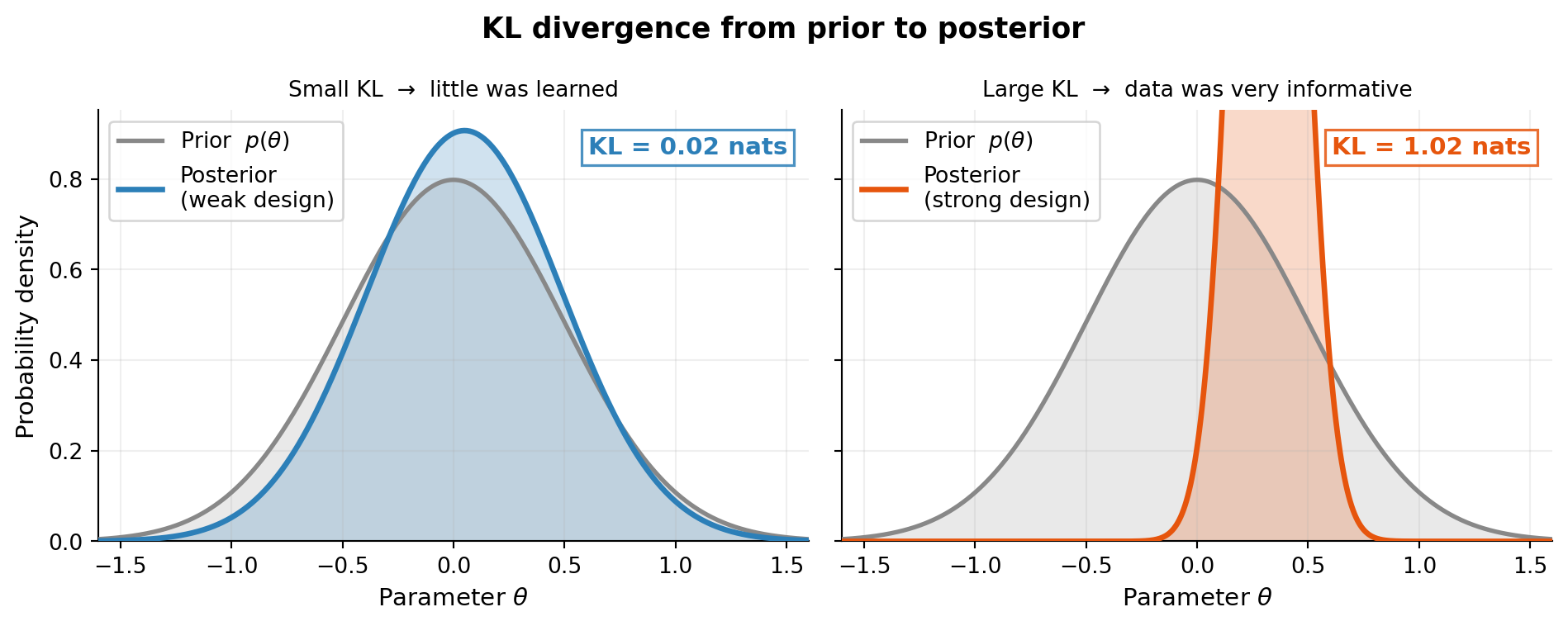
The KL divergence inside the expectation measures, for a specific observation \(\mathbf{y}\), how much the posterior differs from the prior. A large KL means the data forced a big update — the experiment was informative. The outer expectation averages over all observations we might see, giving a design-dependent scalar we can maximize.
NoteEIG = expected KL divergence from prior to posterior
The KL divergence \(\mathrm{KL}(q \| p)\) is zero when \(q = p\) and grows as \(q\) moves away from \(p\). So maximizing EIG drives us toward designs that, on average, produce posteriors as different from the prior as possible.
An Equivalent Expression
Expanding the KL divergence, EIG can be written as a difference of entropies:
\[ \text{EIG}(\mathbf{w}) = H\!\left[p(\boldsymbol{\theta})\right] - \mathbb{E}_{p(\mathbf{y} \mid \mathbf{w})} \!\left[H\!\left[p(\boldsymbol{\theta} \mid \mathbf{y}, \mathbf{w})\right]\right], \]
where \(H\) denotes Shannon entropy. The first term is the prior entropy (fixed, independent of the design). Maximizing EIG therefore minimizes the expected posterior entropy — we want the posterior to be as concentrated as possible, on average.
A third, computationally useful form is:
\[ \text{EIG}(\mathbf{w}) = \mathbb{E}_{p(\boldsymbol{\theta}, \mathbf{y} \mid \mathbf{w})} \!\left[ \log p(\mathbf{y} \mid \boldsymbol{\theta}, \mathbf{w}) - \log p(\mathbf{y} \mid \mathbf{w}) \right]. \]
This is the basis for the double-loop Monte Carlo estimator used in practice (see Bayesian OED: The Double-Loop Estimator).

Linear Gaussian Special Case
For linear Gaussian models the EIG has a closed form involving only the design matrix \(\mathbf{A}\), the prior covariance, and the noise covariance — no simulation required. This makes linear Gaussian benchmarks ideal for validating numerical implementations.
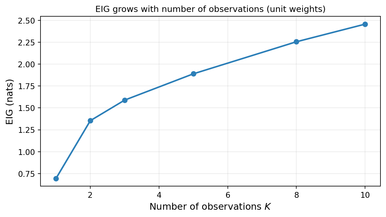
The figure confirms the intuitive result: more observations yield higher EIG, but with diminishing returns — each additional sensor contributes less once the dominant uncertainty directions are already well constrained. Here each sensor receives unit weight (fixed per-sensor precision); if instead a fixed total budget is split equally, spreading it too thinly can actually decrease EIG.
But the number of observations is only part of the story: where the sensors are placed matters just as much. The next figure makes this concrete.

Design A sensors are all clustered near \(x = 0.5\), which gives little discriminating power for the quadratic coefficient \(\theta_2\) — the polynomial basis functions \(1\), \(x\), and \(x^2\) are nearly collinear over that narrow range. Design B spreads sensors across \([0, 1]\), breaking that near-collinearity and achieving far lower posterior variance at every \(K\). The EIG panel confirms the same story: identical sensor counts but very different information yields.
EIG vs. Goal-Oriented OED
EIG measures information gain about the model parameters \(\boldsymbol{\theta}\). When the ultimate interest is a downstream prediction \(q(\boldsymbol{\theta})\) rather than the parameters themselves, optimizing EIG may over-invest in constraining parameter directions that have little effect on \(q\). This motivates goal-oriented OED (covered in Goal-Oriented Bayesian OED).
| Property | EIG / KL-OED | Goal-Oriented OED |
|---|---|---|
| Target | All parameters equally | Specific QoI \(q(\boldsymbol{\theta})\) |
| Utility | Expected KL divergence | Expected risk/deviation of posterior push-forward |
| Closed form | Yes (linear Gaussian) | Yes (linear Gaussian, specific risk measures) |
Key Takeaways
- EIG is the expected KL divergence from the prior to the posterior, averaged over all possible observations.
- Maximizing EIG selects designs that minimize expected posterior entropy.
- For linear Gaussian models, EIG has a closed form and serves as a ground truth for validating numerical approximations.
- When the goal is prediction rather than parameter estimation, goal-oriented OED provides a sharper criterion.
Exercises
Sketch a scenario where maximizing EIG and maximizing information about a specific QoI \(q(\boldsymbol{\theta})\) would lead to different optimal designs. What property of \(q\) makes them diverge?
The EIG formula \(\mathrm{EIG} = H[p(\boldsymbol{\theta})] - \mathbb{E}[H[p(\boldsymbol{\theta}\mid\mathbf{y})]]\) is bounded below by 0. When is it exactly 0? What does that mean physically?
If the prior is very broad (large \(\sigma_\text{prior}\)) and the noise is small, qualitatively what happens to EIG? What if the prior is very tight?
Next Steps
- Bayesian OED: The Double-Loop Estimator — derivation of the double-loop estimator
- Bayesian OED: Gradients and the Reparameterization Trick — C1+C2+C3 gradient derivation
- Bayesian OED: Convergence Verification — using
KLOEDDiagnosticsto validate numerical estimates