From Models to Decisions Under Uncertainty
PyApprox Tutorial Library
Opening tutorial: why computational models need uncertainty quantification, grounded in a composite cantilever beam.
TipDownload Notebook
Learning Objectives
After completing this tutorial, you will be able to:
- Explain why computational models are used to predict complex physical phenomena
- Define a Quantity of Interest (QoI) and explain why predictions are reduced to scalar outputs for decision making
- Identify sources of uncertainty in a computational model and explain why they matter
Prerequisites
Complete Setting Up Your Environment before this tutorial.
Models Predict Complex Physical Phenomena
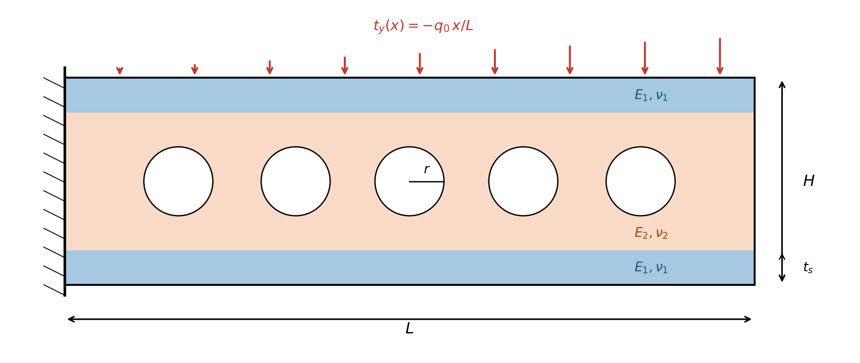
Engineers and scientists routinely use computational models to predict the behavior of systems that are too complex, too expensive, or too dangerous to test exhaustively in the lab. These models underpin critical decisions—from certifying that a structure is safe, to optimizing the design of a new one. But a prediction is only useful if we understand how much to trust it. Uncertainty quantification (UQ) provides the mathematical framework for answering that question. This tutorial is the first in a series introducing core UQ concepts and the PyApprox tools that implement them. We begin with a concrete model problem: a composite cantilever beam with stiff outer skins, a compliant inner core containing circular holes, clamped at one end and loaded on top (see Figure 1).
The beam has three subdomains: stiff skins on the top and bottom (\(E_1, \nu_1\)) and a compliant core with circular holes of radius \(r\) (\(E_2, \nu_2\)). The governing physics is linear elasticity. In each material layer, the stress-strain relationship follows Hooke’s law:
\[ \sigma_{ij} = \lambda \, \varepsilon_{kk} \, \delta_{ij} + 2\mu \, \varepsilon_{ij} \tag{1}\]
where the Lamé parameters \(\lambda\) and \(\mu\) depend on the layer’s Young’s modulus \(E_i\) and Poisson ratio \(\nu_i\). Equilibrium and boundary conditions complete the boundary value problem:
\[ \nabla \cdot \boldsymbol{\sigma} = \vc{0} \;\text{in}\; \Omega, \qquad \vc{u} = \vc{0} \;\text{on}\; \Gamma_D, \qquad \boldsymbol{\sigma} \cdot \vc{n} = \vc{t} \;\text{on}\; \Gamma_N \tag{2}\]
where \(\vc{t} = (0,\, -q_0 x/L)^T\) is the linearly increasing traction on the top surface.
Solving this PDE with a finite element method produces a rich, high-dimensional output: displacement and stress fields over the entire domain. Figure 2 shows the result at fixed (nominal) material properties.

From Full Solutions to Quantities of Interest
The simulation in Figure 2 produces displacement and stress values at thousands of mesh nodes. But an engineer rarely needs the entire field. Instead, they need to answer specific questions that drive decisions:
- Does the beam deflect too much? → Measure the vertical tip displacement \(\delta_{\text{tip}} = u_y(L, H/2)\).
- Will the material yield? → Check the total von Mises stress integrated over the domain, \(\sigma_{\text{tot}} = \int_\Omega \sigma_{\text{vm}}\, dA\).
Each of these is a Quantity of Interest (QoI): a scalar (or low-dimensional) functional of the full model solution that directly informs a decision. In UQ, we focus on characterizing uncertainty in the QoI, not the entire solution field.
The PyApprox beam benchmark returns both QoIs:
\[ q_1 = \delta_{\text{tip}} = u_y(L,\, H/2), \qquad q_2 = \sigma_{\text{tot}} = \int_\Omega \sigma_{\text{vm}}\, dA \tag{3}\]
Throughout these tutorials, we use \(\delta_{\text{tip}}\) as the primary QoI for uncertainty propagation and \(\sigma_{\text{tot}}\) as a secondary QoI that captures global stress information.
Models Are Subject to Uncertainties
So far, we solved the beam at fixed, nominal material properties. But in practice, the inputs to a model are uncertain:
- Parameter uncertainty. The Young’s moduli (\(E_1\), \(E_2\)) and Poisson ratios (\(\nu_1\), \(\nu_2\)) are not known exactly. Manufacturing tolerances, batch-to-batch variability, and limited test data all introduce uncertainty. Figure 3 shows how changing the material stiffness changes the beam’s response: halving the moduli roughly doubles the deflection.

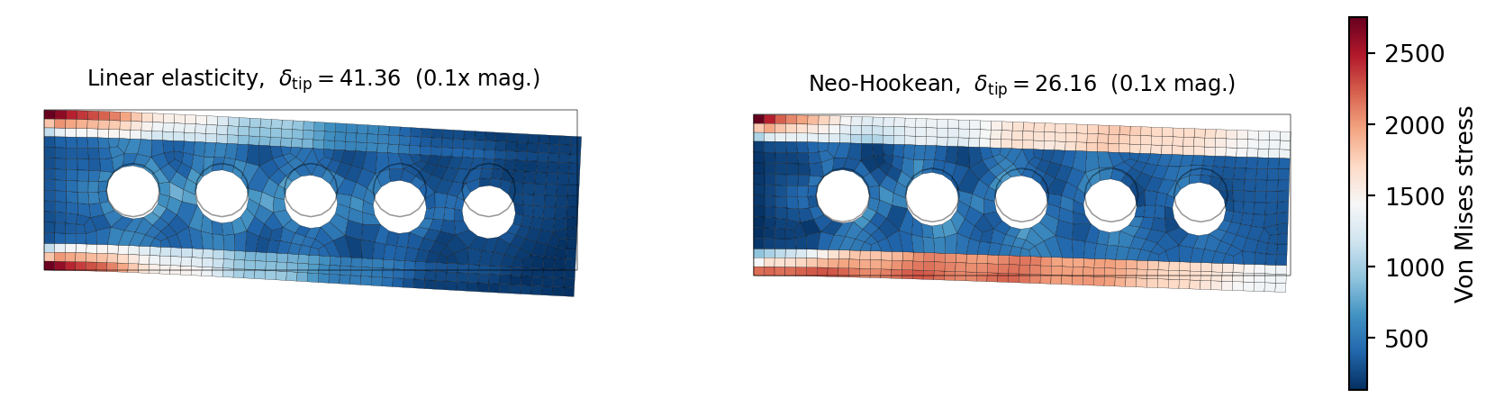
- Model-form uncertainty. The governing equations themselves are approximations. Linear elasticity (Equation 1) assumes small deformations, but under heavy loading the geometry changes enough to stiffen the response. A Neo-Hookean hyperelastic model captures this geometric nonlinearity. Figure 4 shows both models at the same (increased) load: the linear model over-predicts deflection by about 58% because it ignores the stiffening effect of large rotations.
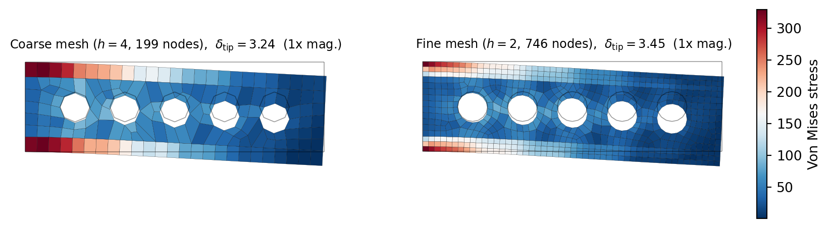
- Numerical uncertainty. The finite element solution depends on the mesh: a coarser mesh is cheaper but less accurate. Figure 5 compares solutions on two meshes; the coarse mesh under-predicts tip deflection by about 6%.
- Data uncertainty. If we calibrate the model against experimental measurements (e.g., measured tip deflection from a lab test), those measurements carry their own noise and systematic errors.
Quantifying the Impact of Uncertainty on the QoI
ImportantThe central challenge
A single model run at nominal inputs gives a single number for \(\delta_{\text{tip}}\). But the true value of \(\delta_{\text{tip}}\) is not a single number—it is a distribution determined by the model uncertainties. Understanding that distribution is the purpose of UQ.
The preceding examples made one thing clear: the QoI is not a single number. Parameter values we cannot pin down exactly, modeling assumptions we know are imperfect, and meshes we know are finite all shift #_{}$ — sometimes by a few percent, sometimes by more than 50%. And these sources of uncertainty do not act in isolation; in a real analysis they compound.
A prediction that ignores this variability is, at best, incomplete — and at worst, dangerously misleading for the decisions it is meant to support. Before we can certify a safety margin, optimize a design, or calibrate against experimental data, we need rigorous answers to questions like: How much can the QoI change given what we do and do not know? Which uncertainties dominate? How confident should we be in the prediction?
Key Takeaways
- Computational models predict complex physical behavior, but decisions are based on specific Quantities of Interest — scalar outputs like tip deflection or integrated stress
- Model predictions are subject to multiple sources of uncertainty: uncertain material parameters, imperfect modeling assumptions, finite mesh resolution, and noisy data
- Each source can significantly change the QoI — parameter variation doubled the deflection, and linear vs. nonlinear constitutive models disagreed by over 50%
- A single prediction at nominal inputs, without accounting for these uncertainties, is insufficient for reliable decision making
- Uncertainty quantification provides the tools to characterize, propagate, and manage these uncertainties — the remaining tutorials introduce those tools
Next Steps
Continue with:
- Random Variables & Distributions – Specifying parameter uncertainty mathematically