---
title: "Monte Carlo Sampling"
subtitle: "PyApprox Tutorial Library"
description: "Estimating QoI statistics by random sampling: variability, sample size effects, and multi-output covariance."
tutorial_type: concept
topic: uncertainty_quantification
difficulty: beginner
estimated_time: 5
render_time: 30
prerequisites:
- forward_uq
- random_variables_distributions
tags:
- uq
- beam
- monte-carlo
- sampling
format:
html:
code-fold: false
code-tools: true
toc: true
execute:
echo: true
warning: false
jupyter: python3
---
::: {.callout-tip collapse="true"}
## Download Notebook
[Download as Jupyter Notebook](notebooks/monte_carlo_sampling.ipynb)
:::
## Learning Objectives
After completing this tutorial, you will be able to:
- Estimate the mean and variance of a QoI using Monte Carlo sampling
- Explain why Monte Carlo estimates are **random** and vary from one set of samples to the next
- Observe that **more samples reduce spread** of Monte Carlo estimates
- Extend Monte Carlo estimation to **multiple QoIs**, including covariance estimation
- Wrap a model for **parallel evaluation** using `make_parallel`
## Prerequisites
Complete [Random Variables & Distributions](random_variables_distributions.qmd) before this tutorial.
## Setup: The Beam Model and Prior
Throughout this tutorial we use a **1D Euler--Bernoulli beam** as a fast surrogate for a more expensive 2D finite-element cantilever beam model. The 1D simplification captures the essential physics --- spatially varying bending stiffness, tip deflection, stress, and curvature --- while running in about 1 ms per sample, making the Monte Carlo experiments below feasible.
The bending stiffness $EI(x)$ is modeled by a two-term Karhunen--Lo\`eve expansion (KLE). The two uncertain parameters $\xi_1, \xi_2 \sim \mathcal{N}(0,1)$ control the dominant modes of the stiffness field. The model returns three QoIs: tip deflection, integrated bending stress, and maximum curvature.
```{python}
import numpy as np
import matplotlib.pyplot as plt
from pyapprox.util.backends.numpy import NumpyBkd
from pyapprox_benchmarks.pde.cantilever_beam import (
    build_cantilever_beam_1d,
)

bkd = NumpyBkd()

# Create problem: KLE beam with 2 uncertain parameters
problem = build_cantilever_beam_1d(bkd, nx=40, num_kle_terms=2)
model = problem.function()
variable = problem.prior()

print(f"Number of uncertain parameters: {model.nvars()}")
print(f"Number of QoIs: {model.nqoi()}")
```
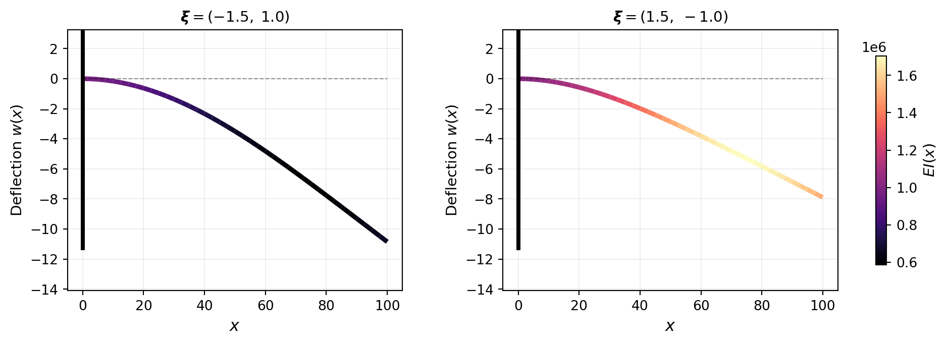
@fig-beam-deflections illustrates how different parameter values change the stiffness field and the resulting deflection. The beam is colored by $EI(x)$: stiffer regions deflect less.
```{python}
#| echo: false
#| fig-cap: "Deflected beam shapes for two different KLE parameter values. Color indicates the spatially varying bending stiffness $EI(x)$. Left: $\\boldsymbol{\\xi} = (-1.5,\\, 1.0)$ produces a stiffness field that is softer near the root, giving larger deflection. Right: $\\boldsymbol{\\xi} = (1.5,\\, -1.0)$ yields a stiffer root region and smaller deflection."
#| label: fig-beam-deflections
from pyapprox_tutorials.figures._forward_uq import plot_beam_deflections
fig, axes = plt.subplots(1, 2, figsize=(13, 3.5),
gridspec_kw={"wspace": 0.3, "right": 0.88})
plot_beam_deflections(problem, bkd, axes[0], axes[1], cbar_fig=fig)
plt.tight_layout()
plt.show()
```
## Sampling the Prior and Evaluating the Model
The Monte Carlo idea is direct: draw $M$ independent samples $\boldsymbol{\theta}^{(1)}, \dots, \boldsymbol{\theta}^{(M)}$ from the prior $\pi(\boldsymbol{\theta})$, evaluate the model at each, and use the results to estimate statistics of the QoI.
```{python}
np.random.seed(42)
M = 50
samples = variable.rvs(M)                          # shape: (2, M)
qoi_values = model(samples)[0]                        # shape: (M,) tip deflection

print(f"Samples shape: {samples.shape}")
print(f"QoI values shape: {qoi_values.shape}")
print(f"Sample mean of tip deflection: "
      f"{bkd.to_float(bkd.mean(qoi_values)):.6f}")
```
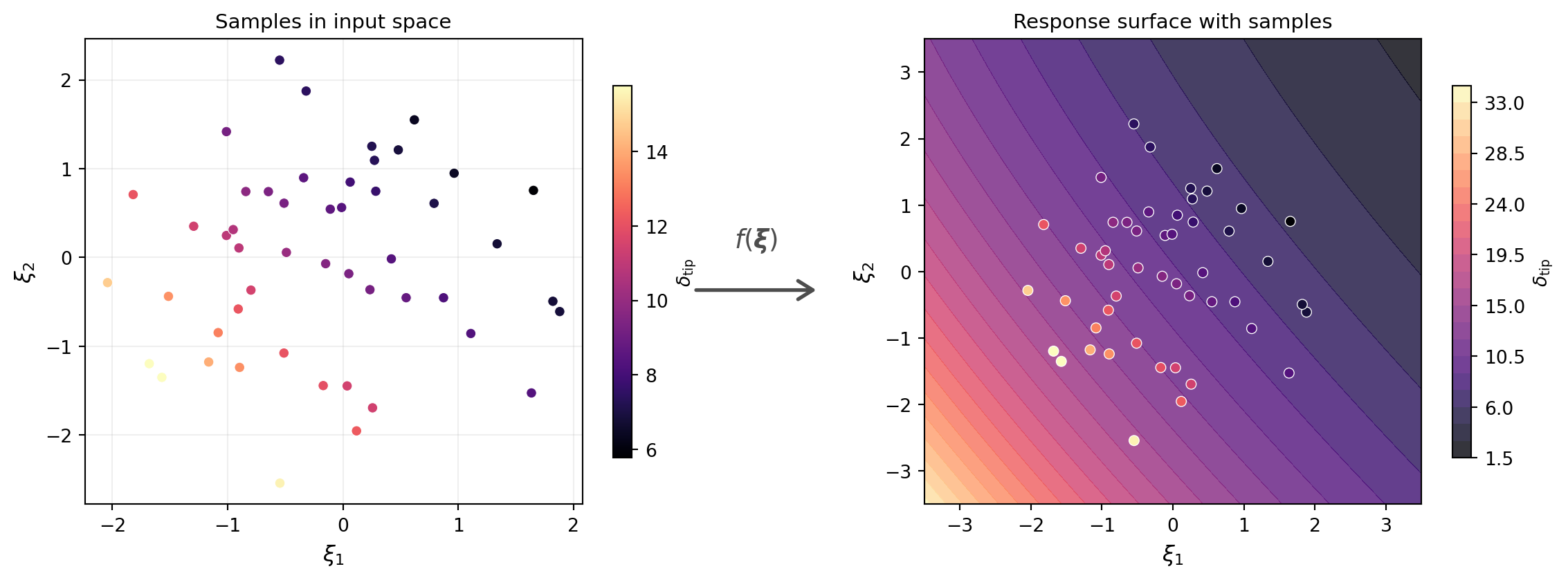
@fig-samples-and-surface shows the samples in input space (left) and the model response surface with the corresponding QoI values overlaid (right). Each point in input space maps to a single value of $\delta_{\text{tip}}$ on the surface.
```{python}
#| echo: false
#| fig-cap: "Left: $M = 50$ samples drawn from the prior in $(\\xi_1, \\xi_2)$ space. Right: the model response surface $\\delta_{\\text{tip}} = f(\\xi_1, \\xi_2)$ with sample QoI values overlaid as colored points."
#| label: fig-samples-and-surface
from pyapprox_tutorials.figures._forward_uq import plot_samples_and_surface
fig, (ax1, ax2) = plt.subplots(1, 2, figsize=(12, 4.5))
plot_samples_and_surface(model, samples, qoi_values, bkd, ax1, ax2, fig=fig)
plt.tight_layout()
plt.subplots_adjust(wspace=0.35)
plt.show()
```
## Accelerating Evaluation with `make_parallel`
Each call to the beam model solves a separate FEM problem. When $M$ is large, these independent solves can run in parallel across CPU cores. PyApprox's `make_parallel` wraps any model satisfying `FunctionProtocol` with a parallel backend:
```{python}
from pyapprox.interface.parallel import make_parallel

model = make_parallel(model, backend="joblib_processes", n_jobs=-1)

print(f"Backend: {model.parallel_backend()}")
print(f"Workers: {model.n_workers()}")
```
The wrapped model has the same interface --- `model(samples)` returns the same results --- but distributes the work across available CPU cores. We reassign `model` so that all subsequent calls automatically benefit from parallelism. For the lightweight 1D beam used here, the speedup is modest; for expensive 2D or 3D FEM solves, it can be substantial.
::: {.callout-note}
## When to parallelize
Parallelization has overhead from spawning workers, serializing data, and collecting results. For models that evaluate in milliseconds (like this 1D beam), the overhead can exceed the computation time. Use `make_parallel` when individual model evaluations take at least tens of milliseconds --- for example, 2D finite-element solves, expensive surrogate evaluations, or models calling external simulation codes.
:::
## Monte Carlo Estimators
Given $M$ samples with QoI values $q^{(1)}, \dots, q^{(M)}$, the **Monte Carlo estimator** of the mean is:
$$
\hat{\mu}_M = \frac{1}{M} \sum_{i=1}^{M} q^{(i)}
$$
and the estimator of the variance is:
$$
\hat{\sigma}^2_M = \frac{1}{M-1} \sum_{i=1}^{M} \left(q^{(i)} - \hat{\mu}_M\right)^2
$$
```{python}
mc_mean = bkd.to_float(bkd.mean(qoi_values))
mc_var = bkd.to_float(bkd.var(qoi_values, ddof=1))

print(f"MC mean estimate (M={M}):     {mc_mean:.6f}")
print(f"MC variance estimate (M={M}): {mc_var:.6f}")
```
These formulas look familiar --- they are just the sample mean and sample variance from introductory statistics. The key question for UQ is: **how accurate are these estimates?**
## Estimates Are Random
To judge the accuracy of Monte Carlo, we need a reference answer. We compute the true mean and variance of the QoI using a high-accuracy deterministic method (quadrature rules are covered in a later tutorial).
```{python}
#| echo: false
from pyapprox.surrogates.quadrature import (
TensorProductQuadratureRule,
gauss_quadrature_rule,
)
nquad = 20
marginals = variable.marginals()
quad_rules = [lambda n, m=m: gauss_quadrature_rule(m, n, bkd) for m in marginals]
quad_rule = TensorProductQuadratureRule(bkd, quad_rules, [nquad] * len(marginals))
quad_pts, quad_wts = quad_rule()
qoi_quad = model(quad_pts)[0]
true_mean = bkd.to_float(bkd.dot(quad_wts, qoi_quad))
true_var = bkd.to_float(
bkd.dot(quad_wts, (qoi_quad - true_mean) ** 2)
)
print(f"True mean (quadrature): {true_mean:.6f}")
print(f"True variance (quadrature): {true_var:.10f}")
```
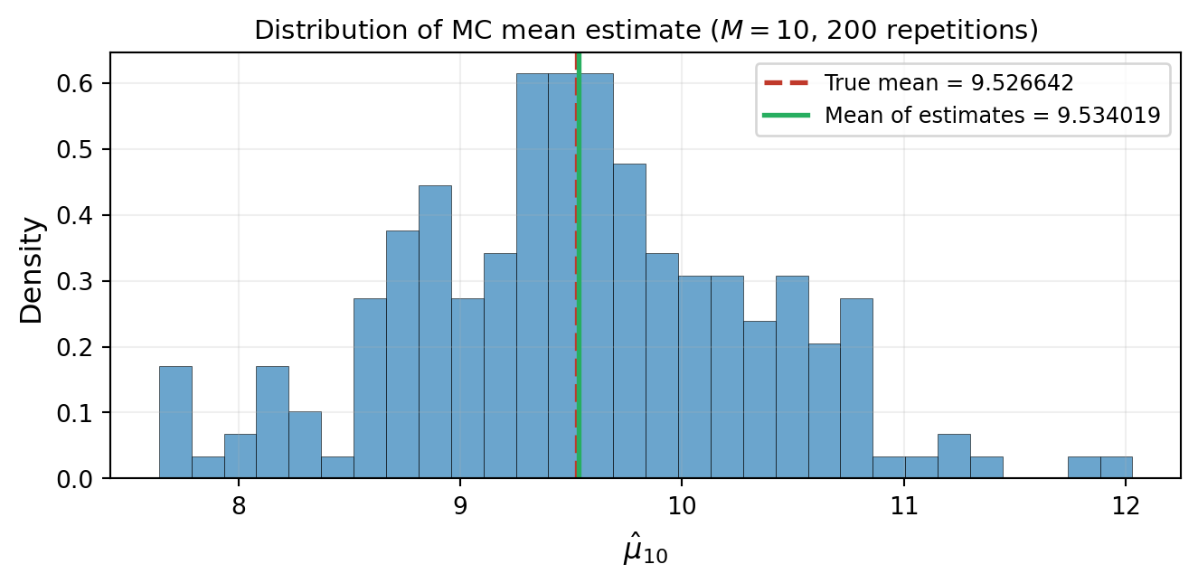
Because the samples are random, the estimates $\hat{\mu}_M$ and $\hat{\sigma}^2_M$ are themselves **random variables**. A different draw of $M$ samples gives a different estimate. @fig-mc-variability-small demonstrates this: we repeat the Monte Carlo experiment 200 times, each with $M = 10$ samples, and collect the resulting mean estimates into a histogram.
```{python}
#| fig-cap: "Variability of the Monte Carlo mean estimate. Each of 200 independent experiments draws $M = 10$ samples and computes $\\hat{\\mu}_{10}$. The histogram shows substantial spread around the true mean (red dashed line)."
#| label: fig-mc-variability-small
n_reps = 200
M_small = 10
means_small = np.empty(n_reps)
for i in range(n_reps):
    np.random.seed(i)
    s = variable.rvs(M_small)
    q = model(s)[0]
    means_small[i] = bkd.to_float(bkd.mean(q))

from pyapprox_tutorials.figures._forward_uq import plot_mc_variability_histogram

fig, ax = plt.subplots(figsize=(7, 3.5))
plot_mc_variability_histogram(means_small, true_mean, n_reps, M_small, ax)
plt.tight_layout()
plt.show()
```
Notice two things. First, the individual estimates are scattered --- some overestimate, some underestimate. Second, the **average of the estimates** (green line) is very close to the true mean (red dashed line). This is not a coincidence.
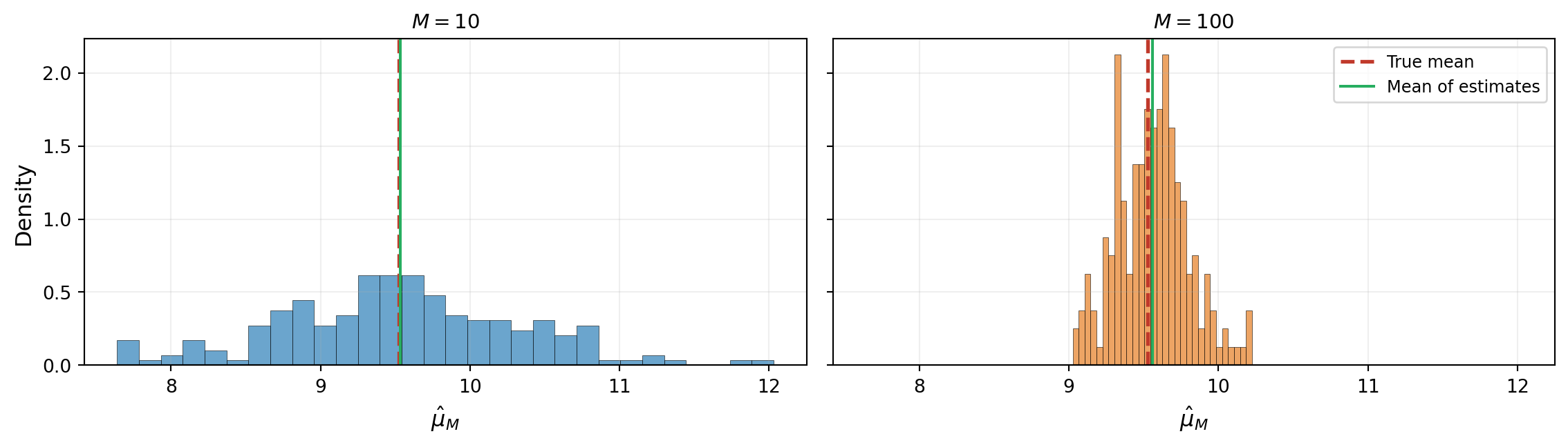
## More Samples, Less Spread
@fig-mc-variability-large repeats the experiment with $M = 100$ samples per repetition. The histogram is dramatically narrower: more samples produce more precise estimates.
```{python}
#| fig-cap: "Same experiment with $M = 100$. The histogram is much narrower: increasing the number of samples reduces the variability of the estimate. The mean of the estimates still matches the true mean."
#| label: fig-mc-variability-large
M_large = 100
means_large = np.empty(n_reps)
for i in range(n_reps):
    np.random.seed(i + 10000)
    s = variable.rvs(M_large)
    q = model(s)[0]
    means_large[i] = bkd.to_float(bkd.mean(q))

from pyapprox_tutorials.figures._forward_uq import plot_mc_variability_comparison

fig, (ax1, ax2) = plt.subplots(1, 2, figsize=(12, 3.5), sharey=True)
plot_mc_variability_comparison(means_small, means_large, true_mean,
                               M_small, M_large, ax1, ax2)
plt.tight_layout()
plt.show()
```
In both cases the average of the estimates matches the true mean. This property has a name: the Monte Carlo mean estimator is **unbiased**.
## Multiple QoIs and Covariance
So far we have tracked a single QoI --- the tip deflection. In practice, a model often produces **several** quantities of interest simultaneously. Our beam model returns three QoIs: the tip deflection $\delta_{\text{tip}}$, the integrated bending stress $\int_0^L \sigma(x)\,dx$, and the maximum absolute curvature $\kappa_{\max}$.
```{python}
np.random.seed(42)
M_multi = 50
samples_multi = variable.rvs(M_multi)
qoi_multi = model(samples_multi)                  # shape: (3, M)

print(f"QoI matrix shape: {qoi_multi.shape}")
print(f"Mean tip deflection:     {bkd.to_float(bkd.mean(qoi_multi[0])):.4f}")
print(f"Mean integrated stress:  {bkd.to_float(bkd.mean(qoi_multi[1])):.2f}")
print(f"Mean max curvature:      {bkd.to_float(bkd.mean(qoi_multi[2])):.6f}")
```
@fig-multi-qoi-scatter shows pairwise scatter plots of the three QoIs. Tip deflection and max curvature are strongly correlated (both increase when the beam is globally softer), while integrated stress is nearly uncorrelated with either --- it depends on where the stiffness varies, not just how much.
```{python}
#| fig-cap: "Pairwise scatter of three QoIs across $M = 50$ samples. Tip deflection and max curvature are highly correlated, while integrated stress is nearly uncorrelated with both."
#| label: fig-multi-qoi-scatter
from pyapprox_tutorials.figures._forward_uq import plot_multi_qoi_scatter

qoi_multi_np = bkd.to_numpy(qoi_multi)
qoi_labels = [
    r"Tip deflection $\delta_{\mathrm{tip}}$",
    r"Integrated stress $\int \sigma\,dx$",
    r"Max curvature $\kappa_{\max}$",
]

fig, axes = plt.subplots(1, 3, figsize=(14, 3.5))
plot_multi_qoi_scatter(qoi_multi_np, qoi_labels, axes)
plt.tight_layout()
plt.show()
```
When multiple QoIs are present, the **covariance matrix** captures how they co-vary:
$$
\hat{\Sigma}_M = \frac{1}{M-1} \sum_{i=1}^{M}
\left(\mathbf{q}^{(i)} - \hat{\boldsymbol{\mu}}_M\right)
\left(\mathbf{q}^{(i)} - \hat{\boldsymbol{\mu}}_M\right)^{\!\top}
$$
where $\mathbf{q}^{(i)} \in \mathbb{R}^{n_{\text{qoi}}}$ and $\hat{\boldsymbol{\mu}}_M$ is the sample mean vector. The diagonal entries are the marginal variances; the off-diagonal entries measure linear dependence between QoIs.
```{python}
cov_matrix = np.cov(qoi_multi_np)
corr_matrix = np.corrcoef(qoi_multi_np)
print("Sample covariance matrix:")
print(cov_matrix)
print("\nCorrelation matrix:")
print(np.array2string(corr_matrix, precision=3))
```
The correlation matrix reveals the structure: tip deflection and max curvature are strongly correlated ($\rho \approx 0.96$) because both are global measures of how much the beam bends. Integrated stress, however, is nearly uncorrelated with both ($\rho \approx 0$) because it depends on the *local* product $EI(x) \cdot \kappa(x)$ --- where the stiffness is high, the stress is high even if curvature is low.
## What Determines Estimation Accuracy?
This tutorial demonstrated two empirical observations:
1. **Monte Carlo estimates are random** --- different samples give different answers
2. **More samples produce more precise estimates** --- the histograms narrowed from $M = {M_small}$ to $M = {M_large}$
But we have not yet explained *how fast* the estimates improve or how to predict the number of samples needed for a given accuracy. These questions require a formal notion of estimator error --- the subject of the next tutorial.
## Exercises
1. Repeat the $M = 10$ vs. $M = {M_large}$ histogram comparison from @fig-mc-variability-large but for the **standard deviation** estimator $\hat{\sigma}_M$ instead of the mean. Does the histogram narrow at the same rate?
2. Using the three-QoI model, repeat the histogram comparison for the off-diagonal covariance entry $\hat{\Sigma}_{01}$ (deflection--stress covariance). How does its variability compare to the mean estimator?
3. **(Challenge)** Compare the convergence of the MC estimate for the deflection--curvature correlation ($\rho_{02} \approx 0.96$) versus the deflection--stress correlation ($\rho_{01} \approx 0$). Which is easier to estimate accurately and why?
## Next Steps
Continue with:
- [Sensitivity Analysis](sensitivity_analysis_concept.qmd) --- Identifying which parameters drive output uncertainty