import numpy as np
import matplotlib.pyplot as plt
from pyapprox.util.backends.numpy import NumpyBkd
from pyapprox_benchmarks.expdesign.lotka_volterra import LotkaVolterraPredictionOEDProblem
from pyapprox.expdesign.data import OEDDataGenerator
from pyapprox.expdesign import (
    GaussianOEDInnerLoopLikelihood,
    create_kl_oed_objective_from_data,
    RelaxedKLOEDSolver,
    RelaxedOEDConfig,
)

np.random.seed(1)
bkd = NumpyBkd()Bayesian OED in Practice: Parameter Estimation for a Predator-Prey System
PyApprox Tutorial Library
Applying EIG-based Bayesian OED to choose when to observe a Lotka-Volterra predator-prey ODE — a nonlinear model where analytic EIG is unavailable.
TipDownload Notebook
Learning Objectives
After completing this tutorial, you will be able to:
- Explain why observation timing matters for identifying Lotka-Volterra parameters
- Construct a nonlinear OED problem using
LotkaVolterraPredictionOEDProblemand the KL-OED API - Generate outer-loop and inner-loop quadrature data from a forward model
- Interpret design weights as a probability measure over candidate observation times
Prerequisites
Complete Bayesian OED: Convergence Verification before this tutorial. That tutorial establishes the API pattern; here we apply it to a problem where no analytical reference exists.
Why Timing Matters for ODE Parameter Identification
The Lotka-Volterra equations describe a predator-prey ecosystem:
\[ \dot{u}_1 = \theta_1 u_1 - \theta_2 u_1 u_2, \qquad \dot{u}_2 = \theta_3 u_1 u_2 - \theta_4 u_2, \]
where \(u_1, u_2\) are prey and predator populations and \(\boldsymbol{\theta} = (\theta_1, \theta_2, \theta_3, \theta_4)\) are growth and interaction rates. We can measure two of the three states at any of several candidate times.
The informativeness of a measurement depends on when it is taken. Early measurements, while the populations are still near their initial conditions, reveal little about the interaction rates \(\theta_2, \theta_3\) — those only become visible once predator-prey cycling has developed. Observations near a population peak or trough carry the most information about the amplitude parameters. OED finds the combination of times that, in expectation across all possible parameter realizations, is most informative.
Setup
oed = LotkaVolterraPredictionOEDProblem(bkd, final_time=50.0)
obs_model = oed.obs_map()   # maps theta -> (nobs_times * 2,)
prior     = oed.inference_problem().prior()  # IndependentJoint over theta
The Model and Observation Structure
# Draw a single prior sample and run the ODE
sample = prior.rvs(1)
full_solution = obs_model.solve_trajectory(sample)[0]   # full ODE trajectory

# Candidate observations: 2 states x T times
observations = obs_model(sample).reshape((2, -1))    # shape (2, T)
Define the Likelihood
noise_std = 0.1
nobs = obs_model.nqoi()
# Each candidate observation has independent additive Gaussian noise
noise_variances = bkd.full((nobs,), noise_std**2)
likelihood = GaussianOEDInnerLoopLikelihood(noise_variances, bkd)
NoteWhy independent diagonal noise?
For ODE state observations, sensor noise is typically uncorrelated across locations and times. The diagonal assumption keeps the log-likelihood computation \(O(K)\) rather than \(O(K^3)\), which matters when \(K\) (the number of candidate observations) is large.
Generate Quadrature Data
The double-loop estimator needs two independent sets of samples from the prior (and the joint prior-noise distribution for the outer loop). The OEDDataGenerator handles this bookkeeping.
data_gen = OEDDataGenerator(bkd)

# Outer loop: joint samples from (theta, epsilon) — used to generate
# synthetic observations y^(m) = f(theta^(m)) + epsilon^(m)
nouter = 3_000
noise_cov_diag = bkd.full((nobs,), noise_std**2)
outerloop_samples, outerloop_weights = data_gen.setup_quadrature_data(
    quadrature_type="MC",
    variable=data_gen.joint_prior_noise_variable(prior, noise_cov_diag),
    nsamples=nouter,
    loop="outer",
)

# Inner loop: prior samples theta^(n) only — used to approximate the evidence
import math
ninner = int(math.sqrt(nouter))    # rule-of-thumb: sqrt of outer budget
innerloop_samples, innerloop_weights = data_gen.setup_quadrature_data(
    quadrature_type="MC",
    variable=prior,
    nsamples=ninner,
    loop="inner",
)
NoteWhy sqrt(N) for the inner loop?
For the EIG estimator the MSE scales as \(O(1/M + 1/N^2)\) where \(M\) is outer and \(N\) is inner. Setting \(N \approx \sqrt{M}\) balances both error sources for a total cost of \(O(M)\) model evaluations.
Evaluate the Forward Model
nparams = prior.nvars()

# Extract prior parameter samples from outer loop
theta_outer = outerloop_samples[:nparams, :]

# Evaluate the observation model at outer and inner parameter samples
outer_shapes = obs_model(theta_outer)     # shape (nobs, nouter)
inner_shapes = obs_model(innerloop_samples)  # shape (nobs, ninner)

# Latent noise samples for the reparameterization trick
latent_samples = outerloop_samples[nparams:, :]  # shape (nobs, nouter)
Create the Objective and Solve
objective = create_kl_oed_objective_from_data(
    noise_variances=noise_variances,
    outer_shapes=outer_shapes,
    inner_shapes=inner_shapes,
    latent_samples=latent_samples,
    bkd=bkd,
    outer_quad_weights=outerloop_weights,
    inner_quad_weights=innerloop_weights,
)

config = RelaxedOEDConfig(maxiter=200, verbosity=0)
solver = RelaxedKLOEDSolver(objective, config)
design_weights, eig = solver.solve()
Interpreting the Design
The output is a probability vector over candidate observation times. Large weight on time \(t_k\) means: observing at \(t_k\) contributes most to learning about the parameters, on average.
from pyapprox_tutorials.figures import plot_lv_design

fig, axes = plt.subplots(1, 2, figsize=(12, 5), sharey=True)
plot_lv_design(axes, oed, design_weights, bkd)
plt.suptitle("Optimal EIG design: Lotka-Volterra", fontsize=12)
plt.tight_layout()
plt.show()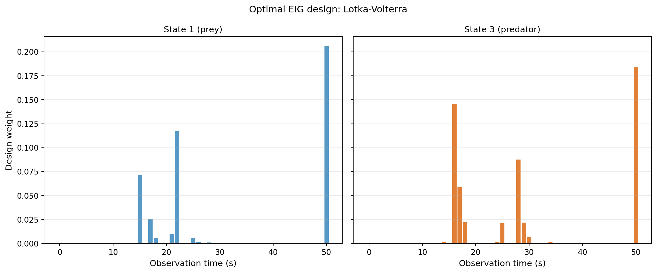
The weights are not uniform — the OED is telling us that some time points are substantially more informative than others. Observations taken while populations are rapidly changing encode more about interaction rates than observations taken at quasi-steady state.
Key Takeaways
- The
create_kl_oed_objective_from_datafactory creates a KL-OED objective from pre-computed model evaluations. Combined withRelaxedKLOEDSolver, this provides an end-to-end OED workflow. - Outer and inner sample counts play distinct roles; the \(\sqrt{M}\) heuristic for inner samples balances bias and variance for minimal total cost.
- Design weights are a probability measure: they tell you how much to invest in each candidate measurement time.
- For nonlinear models, the OED weights depend on the model’s sensitivity structure, which can only be discovered numerically.
Exercises
Re-run with
nouter = 1000andnouter = 50000. How stable are the resulting weight distributions?The noise standard deviation is set to 0.1. Double it to 0.2 and re-solve. Do the optimal times shift, or do the relative weights change?
What happens to the design if you restrict to observing only State 1 (remove State 3)? Does the optimal timing change?
Next Steps
- Design Stability and Convergence — verifying that the design is trustworthy by solving at multiple seeds and budgets
- Goal-Oriented OED: Predator-Prey Prediction — redesign the same experiment to minimise prediction uncertainty rather than parameter estimation error
- Decoupling Data Generation from Optimisation — saving and reusing expensive model evaluations across multiple OED runs