import numpy as np
import matplotlib.pyplot as plt
from pyapprox.util.backends.numpy import NumpyBkd
from pyapprox_benchmarks.pde.cantilever_beam import (
    build_cantilever_beam_2d_linear,
    MESH_PATHS,
)
from pyapprox.surrogates.gaussianprocess import ExactGaussianProcess
from pyapprox.surrogates.kernels.matern import Matern52Kernel
from pyapprox.surrogates.gaussianprocess.fitters import (
    GPFixedHyperparameterFitter,
)

bkd = NumpyBkd()

problem = build_cantilever_beam_2d_linear(bkd, num_kle_terms=1, mesh_path=MESH_PATHS[4])
model     = problem.function()
prior     = problem.prior()
marginals = prior.marginals()
nvars = model.nvars()Adaptive Sampling for Gaussian Processes
PyApprox Tutorial Library
Choose training points that maximally reduce GP posterior uncertainty using greedy Cholesky and IVAR strategies, and compare against space-filling Sobol.
TipDownload Notebook
Learning Objectives
After completing this tutorial, you will be able to:
- Explain why space-filling designs often leave recoverable posterior uncertainty on the table, and how greedy adaptive strategies improve on them
- Describe the Cholesky-greedy criterion: maximise the reduction in log-determinant of the kernel matrix
- Describe the IVAR criterion: minimise the integrated variance over the input space
- Use
CholeskySampler,IVARSampler, andSobolAdaptiveSamplerinterchangeably via theAdaptiveSamplerProtocol - Run a convergence experiment comparing the three strategies on the beam benchmark
Why Adaptive Sampling?
In Building a GP Surrogate we collected training points by simple random sampling from the prior. This is unbiased but wasteful: random samples tend to cluster in high-probability regions, leaving large portions of the input space with high posterior uncertainty that is never resolved.
A smarter approach is adaptive sampling: choose each new training point to maximally reduce the GP’s posterior uncertainty over the entire input space. The two greedy strategies implemented in PyApprox are:
Cholesky-greedy (Pivoted Cholesky): At each step, add the candidate point that maximally increases the log-determinant of the kernel matrix. This is equivalent to pivoted Cholesky factorisation and can be computed incrementally in \(O(N \cdot n)\) time per step (where \(N\) is the number of candidates and \(n\) is the number of points selected so far).
IVAR (Integrated Variance Reduction): At each step, add the candidate point that maximally reduces the integrated posterior variance:
\[ \text{IVAR}(\mathbf{x}^*) = \int \left[\sigma^2(\boldsymbol{\xi}) - \sigma^2_{+\mathbf{x}^*}(\boldsymbol{\xi})\right]\rho(\boldsymbol{\xi})\,d\boldsymbol{\xi} \]
where \(\sigma^2_{+\mathbf{x}^*}\) is the posterior variance after hypothetically adding \(\mathbf{x}^*\) to the training set. This integral reduces to a rank-1 update on the P matrix from UQ with Gaussian Processes.
Both strategies are greedy: they optimise one step at a time without lookahead. This makes them computationally practical while still achieving dramatic improvements over random sampling in practice.
Setup
Candidate Pool
Each sampler selects points from a finite candidate pool drawn in advance from the input distribution. Using a large candidate pool (e.g., 2000 points) ensures good coverage while keeping the greedy search tractable.
N_candidates = 2000
np.random.seed(0)
candidates = prior.rvs(N_candidates)    # (nvars, N_candidates); the pool

# Independent test set for evaluating surrogate accuracy
N_test = 500
np.random.seed(1)
X_test  = prior.rvs(N_test)
y_test  = bkd.to_numpy(model(X_test))[0, :]
The Sampler Protocol
All three samplers implement the same AdaptiveSamplerProtocol:
class AdaptiveSamplerProtocol:
    def set_kernel(self, kernel) -> None: ...
    def select_samples(self, nsamples: int) -> Array: ...   # (nvars, nsamples)
    def add_additional_training_samples(self, X: Array) -> None: ...
This means you can swap strategies with a single line change. Each call to select_samples(n) returns the next n samples; state is preserved between calls so you can extend the training set incrementally without recomputing from scratch.
Cholesky-Greedy Sampler
The pivoted Cholesky factorisation of the kernel matrix selects the sequence of points that best “spans” the reproducing kernel Hilbert space of the GP. At step \(n\) the selected point \(\mathbf{x}_{n+1}\) maximises the residual kernel diagonal:
\[ \mathbf{x}_{n+1} = \argmax_{\mathbf{x} \in \mathcal{C}} \left[k(\mathbf{x}, \mathbf{x}) - \mathbf{k}_n(\mathbf{x})^\top L_n^{-\top} L_n^{-1} \mathbf{k}_n(\mathbf{x})\right] \]
where \(L_n\) is the current Cholesky factor. The residual diagonal is the posterior variance of the GP before conditioning on any output values — this means the Cholesky sampler requires no function evaluations to select points.
from pyapprox.surrogates.gaussianprocess.adaptive.cholesky_sampler import (
    CholeskySampler,
)

# A reference kernel with fixed (reasonable) hyperparameters
ref_kernel = Matern52Kernel([1.0] * nvars, (0.1, 10.0), nvars, bkd)

chol_sampler = CholeskySampler(candidates, bkd)
chol_sampler.set_kernel(ref_kernel)

# Select 30 training points greedily
chol_samples = chol_sampler.select_samples(30)
NoteWarm-starting after kernel update
When hyperparameters are refined on a new training batch, call sampler.set_kernel(updated_kernel) before requesting more samples. The sampler replays the existing pivots with the new kernel and then continues greedy selection. This lets you interleave surrogate fitting and adaptive sampling in an active learning loop.
# Warm-start: update kernel hyperparameters, then add 10 more points
updated_kernel = Matern52Kernel([0.8] * nvars, (0.1, 10.0), nvars, bkd)
chol_sampler.set_kernel(updated_kernel)
extra_samples = chol_sampler.select_samples(10)   # 10 new points under new kernel
IVAR Sampler
IVAR selects the point with the largest integrated variance reduction. It requires the P matrix — the same kernel double-integral used in the UQ statistics — as additional input:
\[ P_{ij} = \int k(\boldsymbol{\xi}, \boldsymbol{\xi}^{(i)}) k(\boldsymbol{\xi}, \boldsymbol{\xi}^{(j)}) \rho(\boldsymbol{\xi})\,d\boldsymbol{\xi} \]
We approximate the P matrix with Monte Carlo quadrature using samples from the prior.
from pyapprox.surrogates.gaussianprocess.adaptive.ivar_sampler import (
    IVARSampler,
)

def compute_P_mc(kernel, candidates, prior, bkd, nquad=5000):
    """Approximate P matrix via Monte Carlo with prior samples."""
    np.random.seed(123)
    quad_pts = prior.rvs(nquad)                # (nvars, nquad)
    K_qc = kernel(quad_pts, candidates)        # (nquad, ncandidates)
    return (K_qc.T @ K_qc) / nquad

P = compute_P_mc(ref_kernel, candidates, prior, bkd)

ivar_sampler = IVARSampler(candidates, bkd)
ivar_sampler.set_kernel(ref_kernel)
ivar_sampler.set_P(P)

ivar_samples = ivar_sampler.select_samples(30)
The IVAR criterion is slightly more expensive per step than Cholesky because it involves a rank-1 update to a matrix solve, but it directly optimises the quantity we care about for UQ — integrated posterior variance.
Sobol Sampler (Baseline)
The SobolAdaptiveSampler generates a low-discrepancy Sobol sequence mapped to the input bounds. It implements the same protocol but ignores the kernel entirely. We use it as a strong space-filling baseline.
from pyapprox.surrogates.gaussianprocess.adaptive.sobol_sampler import (
    SobolAdaptiveSampler,
)

def map_uniform_to_marginals(samples_01, marginals, bkd):
    """Map [0,1]^d Sobol samples to physical space via per-marginal inverse CDF."""
    mapped = bkd.zeros_like(samples_01)
    for d in range(samples_01.shape[0]):
        mapped[d:d+1, :] = marginals[d].invcdf(samples_01[d:d+1, :])
    return mapped

# Sobol in [0,1]^d, then transform to prior distribution
sobol_sampler = SobolAdaptiveSampler(nvars, bkd)
sobol_samples = sobol_sampler.select_samples(30)
# Map [0,1]^d to prior distribution using the inverse CDF
sobol_samples_mapped = map_uniform_to_marginals(sobol_samples, marginals, bkd)
Visualising the Sample Designs
For 2D projections, we can see how the three strategies distribute their points.
from pyapprox_tutorials.figures._gp import plot_sample_designs

strategies = [
    (bkd.to_numpy(chol_samples), "#1A5276", "Cholesky-greedy"),
    (bkd.to_numpy(ivar_samples), "#117A65", "IVAR"),
    (bkd.to_numpy(sobol_samples_mapped), "#7D3C98", "Sobol (mapped)"),
]

fig, axes = plt.subplots(1, 3, figsize=(12, 4))
plot_sample_designs(axes, strategies)
plt.tight_layout()
plt.show()
Convergence Experiment
We now run a systematic convergence study: for each strategy and each training budget \(N \in \{10, 15, 20, 30, 40, 60, 80, 100\}\), we:
- Select \(N\) training points using the strategy
- Evaluate the beam model at those points
- Fit a GP (fixed hyperparameters for comparability)
- Compute the relative \(L_2\) error on the test set
Because the greedy samplers are deterministic, each budget is simply an extension of the previous one — no re-evaluation is needed.
from pyapprox.surrogates.gaussianprocess.fitters import (
    GPFixedHyperparameterFitter,
)

budgets = [10, 15, 20, 30, 40, 60, 80, 100]

def _fit_and_evaluate(X_tr, y_tr, kernel):
    """Fit GP with fixed hyperparameters and return L2 error on test set."""
    gp = ExactGaussianProcess(kernel, nvars=nvars, bkd=bkd, nugget=1e-6)
    gp.hyp_list().set_all_inactive()
    fitter = GPFixedHyperparameterFitter(bkd)
    result = fitter.fit(gp, X_tr, y_tr)
    fitted_gp = result.surrogate()
    y_pred = bkd.to_numpy(fitted_gp.predict(X_test))[0, :]
    return np.linalg.norm(y_test - y_pred) / np.linalg.norm(y_test)

# ---- Cholesky convergence ----
chol_sampler2 = CholeskySampler(candidates, bkd)
chol_sampler2.set_kernel(ref_kernel)

chol_errors = []
prev_n = 0
X_chol_accum = None
y_chol_accum = None
for n in budgets:
    new_pts = chol_sampler2.select_samples(n - prev_n)
    new_vals = model(new_pts)[:1, :]
    X_chol_accum = new_pts if X_chol_accum is None else bkd.hstack([X_chol_accum, new_pts])
    y_chol_accum = new_vals if y_chol_accum is None else bkd.hstack([y_chol_accum, new_vals])
    chol_errors.append(_fit_and_evaluate(X_chol_accum, y_chol_accum, ref_kernel))
    prev_n = n

# ---- IVAR convergence ----
ivar_sampler2 = IVARSampler(candidates, bkd)
ivar_sampler2.set_kernel(ref_kernel)
ivar_sampler2.set_P(P)

ivar_errors = []
prev_n = 0
X_ivar_accum = None
y_ivar_accum = None
for n in budgets:
    new_pts = ivar_sampler2.select_samples(n - prev_n)
    new_vals = model(new_pts)[:1, :]
    X_ivar_accum = new_pts if X_ivar_accum is None else bkd.hstack([X_ivar_accum, new_pts])
    y_ivar_accum = new_vals if y_ivar_accum is None else bkd.hstack([y_ivar_accum, new_vals])
    ivar_errors.append(_fit_and_evaluate(X_ivar_accum, y_ivar_accum, ref_kernel))
    prev_n = n

# ---- Sobol (random seed repeated for each budget — not incremental) ----
sobol_errors = []
for n in budgets:
    sobol_s2 = SobolAdaptiveSampler(nvars, bkd)
    pts_raw  = sobol_s2.select_samples(n)
    pts      = map_uniform_to_marginals(pts_raw, marginals, bkd)
    vals     = model(pts)[:1, :]
    sobol_errors.append(_fit_and_evaluate(pts, vals, ref_kernel))
from pyapprox_tutorials.figures._gp import plot_gp_sampling_convergence
fig, ax = plt.subplots(figsize=(7, 4.5))
plot_gp_sampling_convergence(ax, budgets, chol_errors, ivar_errors, sobol_errors)
plt.tight_layout()
plt.show()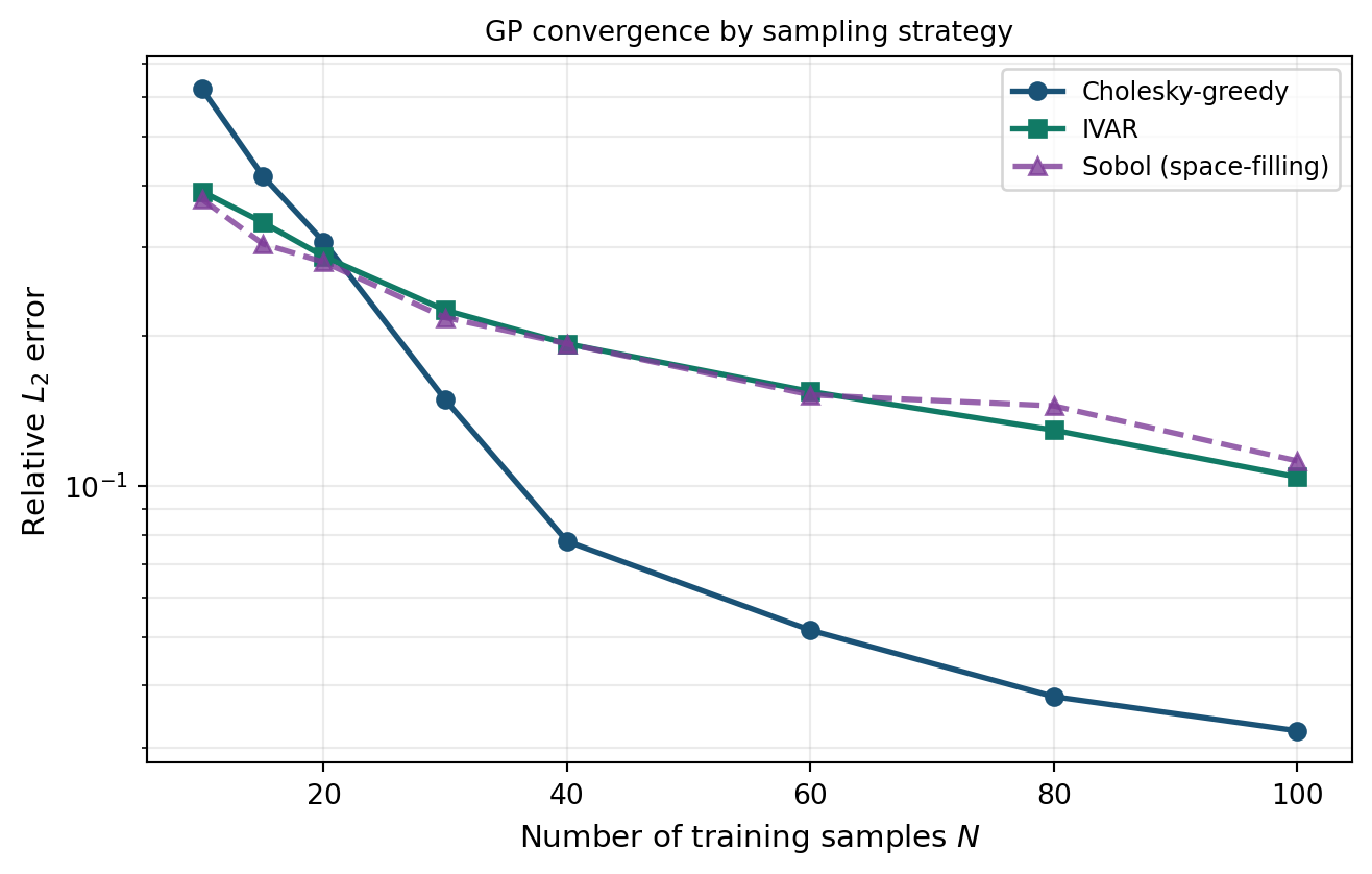
The adaptive strategies typically achieve the same accuracy as Sobol with significantly fewer model evaluations. The exact gap depends on the smoothness of the model and the dimension of the input space; for higher-dimensional problems the advantage of adaptive strategies grows.
Active Learning Loop
In practice, hyperparameters are not known in advance. A standard workflow is to interleave adaptive sampling with hyperparameter re-fitting in batches:
from pyapprox.surrogates.gaussianprocess.fitters import (
    GPMaximumLikelihoodFitter,
)

# --- Active learning loop with Cholesky-greedy ---
batch_size   = 10
n_batches    = 5
loop_sampler = CholeskySampler(candidates, bkd)
loop_kernel  = Matern52Kernel([1.0] * nvars, (0.1, 10.0), nvars, bkd)
loop_sampler.set_kernel(loop_kernel)

X_loop = None
y_loop = None
loop_errors = []

for batch in range(n_batches):
    # 1. Select next batch of training points
    new_pts  = loop_sampler.select_samples(batch_size)
    new_vals = model(new_pts)[:1, :]

    X_loop = new_pts  if X_loop is None else bkd.hstack([X_loop, new_pts])
    y_loop = new_vals if y_loop is None else bkd.hstack([y_loop, new_vals])

    # 2. Fit GP and optimise hyperparameters
    loop_gp = ExactGaussianProcess(loop_kernel, nvars=nvars, bkd=bkd, nugget=1e-6)
    ml_fitter  = GPMaximumLikelihoodFitter(bkd)
    loop_result = ml_fitter.fit(loop_gp, X_loop, y_loop)
    loop_gp     = loop_result.surrogate()

    # 3. Update sampler kernel with refined hyperparameters
    loop_sampler.set_kernel(loop_gp.kernel())

    # 4. Evaluate accuracy
    y_pred = bkd.to_numpy(loop_gp.predict(X_test))[0, :]
    err    = np.linalg.norm(y_test - y_pred) / np.linalg.norm(y_test)
    loop_errors.append(err)

    n_total = (batch + 1) * batch_size
Key Takeaways
- Space-filling designs (Sobol, Latin hypercube) are simple and robust but do not use kernel information to choose informative points
- Cholesky-greedy selection maximises information gain per step via an incremental pivoted Cholesky factorisation; it is fast (no model evaluations needed to rank candidates) and supports warm-starting after kernel updates
- IVAR directly minimises integrated posterior variance — the quantity most relevant for UQ — and often outperforms Cholesky on smooth models at the cost of computing the P matrix
- All three strategies implement the same
AdaptiveSamplerProtocol, making them interchangeable with a single line change - An active learning loop interleaves adaptive sampling with hyperparameter refitting, so the sampler continuously adapts as more data are collected
Exercises
In the convergence experiment, add a random sampling baseline (draw \(N\) points iid from the prior at each budget). How much worse is it compared to Sobol?
The Cholesky sampler uses a reference kernel with fixed hyperparameters to rank candidates. Experiment with different length scales (\(0.3\) vs \(3.0\)) for the reference kernel. How sensitive is the convergence to this choice?
Extend the active learning loop to use IVAR instead of Cholesky. The P matrix must be recomputed each time
set_kernelis called. Does the extra cost pay off in lower error at a given budget?Try
set_weight_functionon theCholeskySamplerto bias sampling towards regions where \(|\xi_1| > 1\) (the tails of the Gaussian). Does this improve tail accuracy at the cost of centre accuracy?
Next Steps
- Multi-Output Gaussian Processes — Extend adaptive sampling to multi-fidelity settings using
MultiOutputIVARSampler - Building a GP Surrogate — Review GP fitting basics
- UQ with Gaussian Processes — Use the P matrix from IVAR sampling to also compute analytical moments