Multi-Output Approximate Control Variates
PyApprox Tutorial Library
Why estimating several quantities of interest jointly with multi-fidelity corrections improves each individual estimate — the key non-obvious insight of multi-output ACV.
TipDownload Notebook
Learning Objectives
After completing this tutorial, you will be able to:
- State the key non-obvious insight: estimating QoI \(s\) together with other QoIs reduces the variance of the QoI \(s\) estimate compared to estimating it alone
- Explain intuitively why cross-QoI covariances provide additional signal for each individual QoI
- Identify the regime in which MOACV outperforms SOACV (multiple runs of scalar ACV)
- Read and interpret an MOACV vs SOACV variance reduction comparison
Prerequisites
Complete General ACV Concept before this tutorial.
The Surprising Benefit of Estimating Together
Plain joint MC does not improve any individual QoI’s variance: the \(s\)-th diagonal entry of the MC covariance matrix is \(\boldsymbol{\Sigma}_{0,ss}/N\), identical to running scalar MC for that QoI alone.
With multi-fidelity corrections, the situation changes. Estimating all QoIs together with ACV corrections can substantially improve each individual QoI’s estimate compared to running one scalar ACV per QoI independently. This is the central, non-obvious claim of multi-output ACV.
Why? In scalar ACV, the correction term for QoI \(s\) is \(\eta_s \bigl(\hat{\mu}_{\alpha,s}^* - \hat{\mu}_{\alpha,s}\bigr)\). The optimal weight \(\eta_s^*\) uses only the covariance between QoI \(s\) corrections and the QoI \(s\) HF estimate.
In multi-output ACV (MOACV), the weight matrix \(\mathbf{H}^* \in \mathbb{R}^{S \times SM}\) couples every QoI’s estimate to the corrections of every QoI of every LF model. Specifically, the correction for QoI \(s\) can include a term proportional to \(\hat{\mu}_{\alpha,t}^* - \hat{\mu}_{\alpha,t}\) for \(t \neq s\) if those corrections are correlated with the QoI \(s\) HF estimation error. This cross-QoI covariance is free information that scalar ACV leaves on the table.
Intuition with a Two-QoI Example
Suppose model \(f_0\) produces outputs \((f_{0,1}, f_{0,2})\) that are highly correlated. We have a cheap LF model \(f_1\) that closely tracks both outputs.
SOACV (scalar per QoI): Estimate \(\mu_{0,1}\) using corrections from \(f_{1,1}\) only. Estimate \(\mu_{0,2}\) using corrections from \(f_{1,2}\) only. Each scalar ACV uses \(M\cdot S = 2\) LF outputs (one per model per QoI, but only matching-output corrections).
MOACV (joint): Estimate \(\mu_{0,1}\) using corrections from both \(f_{1,1}\) and \(f_{1,2}\) simultaneously. Because \(f_{0,1}\) and \(f_{0,2}\) are correlated, the noise in estimating \(\mu_{0,1}\) carries information about the noise in \(f_{1,2}\)’s correction. The optimal weight matrix \(\mathbf{H}^*\) exploits this: if the \(f_{1,2}\) correction is large and positive, and the two outputs are correlated, this is evidence that the \(f_{1,1}\) correction is also too large — so downweight it. This extra signal can only help, never hurt.
Formally, the MOACV optimal covariance is always \(\leq\) the SOACV covariance in the positive-semidefinite sense, with equality only when QoI outputs are uncorrelated across the hierarchy.
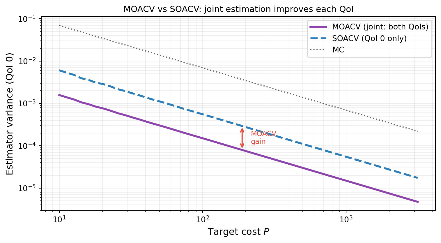
MOACV vs SOACV: The Key Figure
Figure 1 shows the estimator variance for QoI 0 under MOACV, SOACV, and plain MC across a range of target costs, using the three-model two-QoI benchmark. SOACV runs a separate scalar ACV for QoI 0, ignoring the information in QoI 1. MOACV estimates both QoIs jointly and is uniformly better for QoI 0.
The MOACV curve is uniformly below the SOACV curve. At any budget, estimating QoI 0 alongside QoI 1 is strictly better for QoI 0 than estimating QoI 0 alone.
When Does MOACV Win Most?
The gain from joint estimation depends on the cross-QoI structure:
| Regime | MOACV gain over SOACV |
|---|---|
| QoI outputs are uncorrelated across models | Zero (MOACV = SOACV) |
| Strong within-model cross-QoI correlation | Large gain |
| Different LF models better predict different QoIs | Substantial gain |
| QoIs have very different signal-to-noise ratios | Moderate gain |
The gain is zero only when \([\boldsymbol{\Sigma}]_{\alpha s, \beta t} = 0\) for all \(s \neq t\) (all cross-QoI covariances vanish). In this case the optimal weight matrix \(\mathbf{H}^*\) is block-diagonal and MOACV decouples into \(S\) independent scalar ACVs. In all other cases, there is a strict gain.
A Useful Mental Model
Think of MOACV as extending the Schur complement variance reduction from the general ACV formula. In scalar ACV, the reduction is \(\sigma_{0\Delta}^\top \Sigma_{\Delta\Delta}^{-1} \sigma_{0\Delta}\), which uses correlations between \(\hat{\mu}_0(\mathcal{Z}_0)\) and each correction \(\Delta_\alpha\).
In MOACV, the vector of corrections \(\boldsymbol{\Delta}\) now includes corrections for all QoIs of all LF models. This means the Schur complement exploits both cross-model (different \(\alpha\)) and cross-QoI (different \(s\)) correlations. The expanded \(\boldsymbol{\Delta}\) vector is strictly more informative, so the Schur complement is larger, and the variance reduction is at least as large as SOACV.
Key Takeaways
- The central insight: jointly estimating multiple QoIs with ACV corrections reduces each individual QoI’s variance compared to separate scalar ACVs, whenever cross-QoI corrections are correlated
- The gain is structural: the MOACV weight matrix \(\mathbf{H}^*\) has more non-zero entries than the SOACV weight matrix, enabling it to exploit cross-QoI signal
- The gain vanishes only when all cross-QoI population covariances are zero — a rare edge case for physically meaningful model ensembles
- MOACV is always at least as good as SOACV; the choice never hurts
Exercises
Suppose you have two perfectly correlated QoIs: \(f_{0,2} = f_{0,1}\) and \(f_{1,2} = f_{1,1}\). Does MOACV give any gain over SOACV? Explain using the cross-QoI covariance structure.
Suppose the two QoIs are perfectly anti-correlated: \(f_{0,2} = -f_{0,1}\) and similarly for \(f_1\). Does MOACV gain over SOACV? Sketch the structure of \(\mathbf{H}^*\).
From Figure 1, estimate the percentage improvement in QoI 0 variance at cost \(P = 100\). Does the relative improvement grow or shrink as budget increases?
Next Steps
- Multi-Output ACV Analysis — Derive the MOACV optimal weight matrix \(\mathbf{H}^*\) and the resulting minimum covariance
- API Cookbook — Run MOACV and SOACV end-to-end and confirm the improvement numerically
Tip
Ready to try this? See API Cookbook → Multi-Output Estimation.
References
[DWBG2024] D. Schaden, E. Ullmann, R. Butler, J. Jakeman. Multi-output approximate control variates. 2024. arXiv:2310.00125
[RM1985] R. Y. Rubinstein and R. Marcus. Efficiency of multivariate control variates in Monte Carlo simulation. Operations Research, 33(3):661–677, 1985.