Note
Go to the end to download the full example code
Multi-level and Multi-index Collocation
Thsi tutorial introduces multi-level [TJWGSIAMUQ2015] and multi-index collocation [HNTTCMAME2016]. It assumes knowledge of the material covered in Tensor-product Interpolation and Sparse Grids.
Models often utilize numerical discretizations to solve the equations governing the system dynamics. For example, finite-elements, spectral collocation, etc are often used to solve partial differential equations. Convergence studies demonstrates how the numerical discretization, specifically the spatial mesh discretization and time-step, of a spectral collocation model of transient advection diffusion effects the accuracy of the model output.
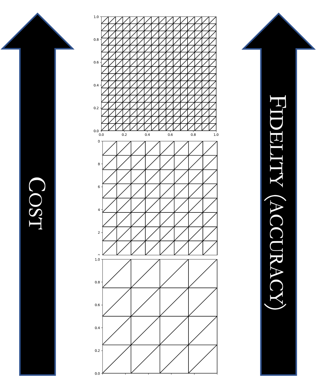
A multi-level hierarchy formed by increasing mesh discretizations. |
An observation
Multilevel collocation was introduced to reduce the cost of building surrogates of models when a one-dimensional hierarchy of numerical discretizations of a model \(f_\alpha(\rv), \alpha=0,1,\ldots\) are available such that
if \(\alpha^\prime < \alpha.\) and the work \(W_\alpha\) increases with fidelity.
Multilevel collocation can be implemented by modifying sparse grid interplation developed for a single model fidelity. The modification is based on the observation that the discrepancy between two consecutive models and the lower-fidelity model will be computationally cheaper to approximate than higher-fidelity model.
The following code demonstrates this observation for a simple 1D model with two numerical discretizations
import numpy as np
from functools import partial
from scipy import stats
from pyapprox.variables.joint import IndependentMarginalsVariable
import matplotlib.pyplot as plt
from pyapprox.surrogates.approximate import adaptive_approximate
from pyapprox.surrogates.interp.adaptive_sparse_grid import (
    tensor_product_refinement_indicator, isotropic_refinement_indicator,
    variance_refinement_indicator)
from pyapprox.variables.transforms import ConfigureVariableTransformation
from pyapprox.interface.wrappers import MultiIndexModel

def fun(eps, zz):
    return np.cos(np.pi*(zz[0]+1)/2+eps)[:, None]


funs = [partial(fun, 0.25), partial(fun, 0)]
variable = IndependentMarginalsVariable([stats.uniform(-1, 2)])
ranges = variable.get_statistics("interval", 1.0).flatten()
zz = np.linspace(*ranges, 101)
axs = plt.subplots(1, 3, figsize=(3*8, 6), sharey=True)[1]

def build_tp(fun, max_level_1d):
    tp = adaptive_approximate(
        fun, variable, "sparse_grid",
        {"refinement_indicator": tensor_product_refinement_indicator,
         "max_level_1d": max_level_1d,
         "univariate_quad_rule_info": None}).approx
    return tp

lf_approx = build_tp(funs[0], 2)
axs[0].plot(zz, funs[0](zz[None, :]), 'k', label=r"$f_0$")
axs[0].plot(zz, funs[1](zz[None, :]), 'r', label=r"$f_1$")
axs[0].plot(lf_approx.samples[0], lf_approx.values[:, 0], 'ko')
axs[0].plot(zz, lf_approx(zz[None])[:, 0], 'g:', label=r"$f_{0,\mathcal{I}_0}$")
axs[0].legend(fontsize=18)

hf_approx = build_tp(funs[1], 1)
axs[1].plot(zz, funs[1](zz[None, :]), 'r', label=r"$f_1$")
axs[1].plot(hf_approx.samples[0], hf_approx.values[:, 0], 'ro')
axs[1].plot(zz, hf_approx(zz[None])[:, 0], ':', color='gray',
            label=r"$f_{1,\mathcal{I}_1}$")
axs[1].legend(fontsize=18)

def discrepancy_fun(fun1, fun0, zz):
    return fun1(zz)-fun0(zz)

discp_approx = build_tp(partial(discrepancy_fun, funs[1], lf_approx), 1)
axs[2].plot(zz, funs[1](zz[None, :]), 'r', label=r"$f_1$")
axs[2].plot(zz, funs[1](zz[None, :])-funs[0](zz[None, :]), 'k',
            label=r"$\delta=f_1-f_0$")
axs[2].plot(discp_approx.samples[0], discp_approx.values[:, 0], 'ko')
axs[2].plot(zz, discp_approx(zz[None, :]),
            'g:', label=r"$\delta_{\mathcal{I}_1}$")
axs[2].plot(zz, lf_approx(zz[None])+discp_approx(zz[None, :]),
            'b:', label=r"$f_{0,\mathcal{I}_1}+\delta_{\mathcal{I}_1}$")
[ax.set_xlabel(r"$z$") for ax in axs]
_ = axs[2].legend(fontsize=18)
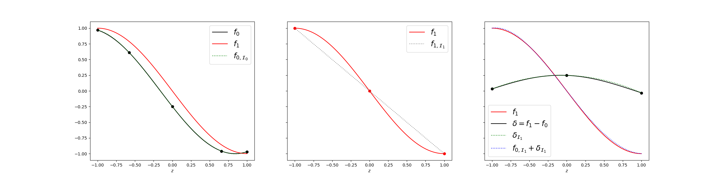
The left plot shows that using 5 samples of the low-fidelity model produces an accurate approximation of the low-fidelity model, but it will be a poor approximation of the high fidelity model in the limit of infinite low-fidelity data. The middle plot shows three samples of the high-fidelity model also produces a poor approximation, but if more samples were added the approximation would coverge to the high-fidelity model. In contrast the right plot shows that 5 samples of the low-fideliy model plus three samples of the high-fidelity model produces a good approximation of the high-fidelity model.
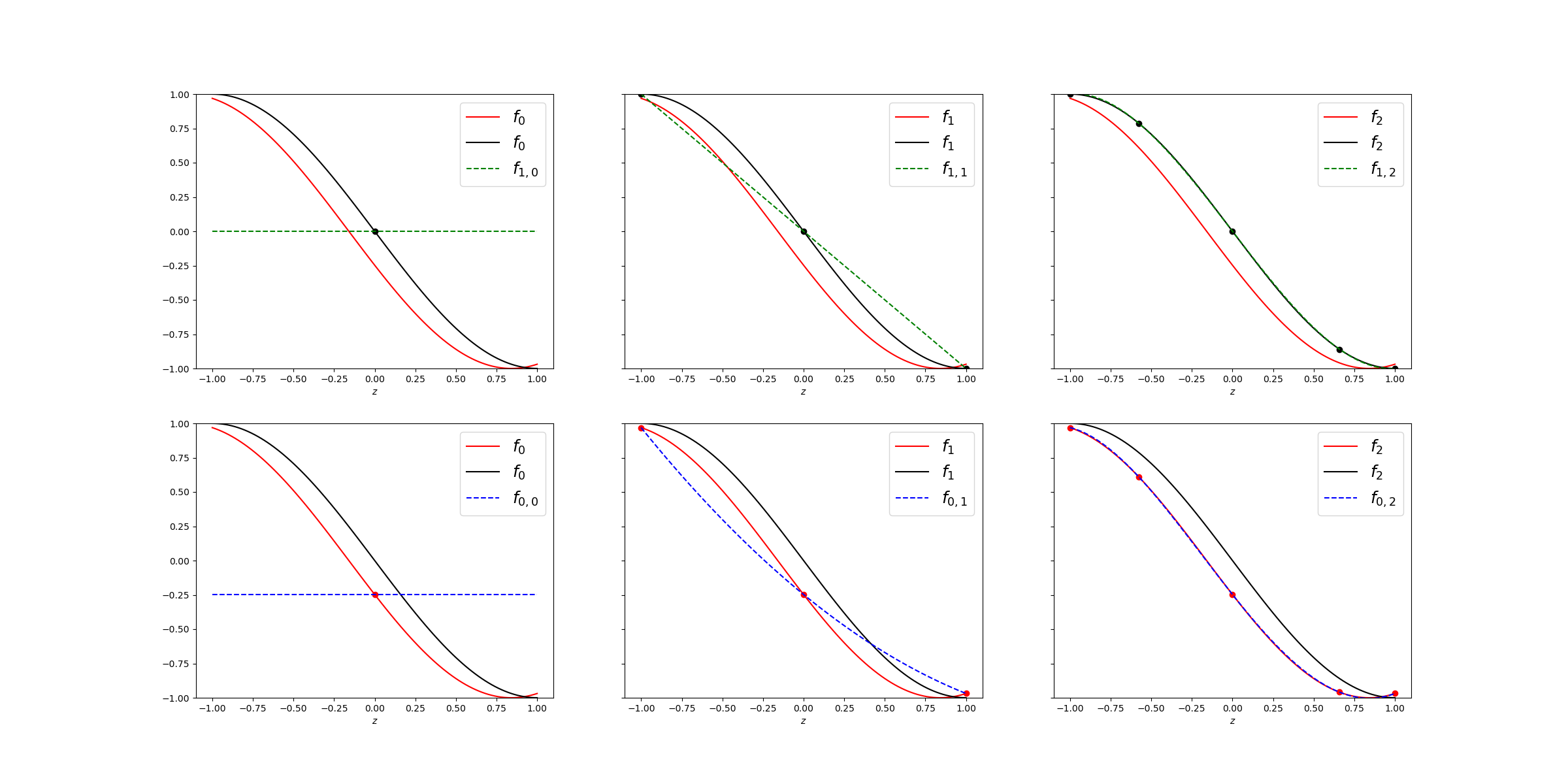
The following code plots different interpolations \(f_{\alpha,\beta}\) of \(f_\alpha\) for various \(\alpha\) and number of interpolation points (controled by \(\beta\)). Instead of building each interpolant with a custom function, we just build a multi-index sparse grid that uses a tensor-product refinement criterion to define the set \(\mathcal{I}=\{[\alpha,\beta]:\alpha \le l_0, \; \beta\le l_1\}\)
max_level = 2
nvars = 1
config_values = [np.asarray([0.25, 0])]
# config_values = [np.asarray([0.25, 0.125, 0])]
config_var_trans = ConfigureVariableTransformation(config_values)


def setup_model(config_values):
    eps = config_values[0]
    return partial(fun, eps)

mi_model = MultiIndexModel(setup_model, config_values)

# cannot let max_level_1d for configure variables be larger
# than number of configure variables
max_level_1d = [max_level, len(config_values[0])-1]  # [l_0, l_1]

fig, axs = plt.subplots(
    max_level_1d[1]+1, max_level_1d[0]+1,
    figsize=((max_level_1d[0]+1)*8, (max_level_1d[1]+1)*6),
    sharey=True)

tp_approx = adaptive_approximate(
    mi_model, variable, "sparse_grid",
    {"refinement_indicator": tensor_product_refinement_indicator,
     "max_level_1d": max_level_1d,
     "config_variables_idx": nvars,
     "config_var_trans": config_var_trans,
     "univariate_quad_rule_info": None}).approx

from pyapprox.surrogates.interp.sparse_grid import (
    get_subspace_values, evaluate_sparse_grid_subspace)
fun_colors = ['r', 'k', 'cyan']
approx_colors = ['b', 'g', 'pink']
for ii, subspace_index in enumerate(tp_approx.subspace_indices.T):
    subspace_values = get_subspace_values(
        tp_approx.values, tp_approx.subspace_values_indices_list[ii])
    jj, kk = subspace_index
    subspace_samples = tp_approx.samples_1d[0][jj]
    ax = axs[max_level_1d[1]-kk, jj]
    ax.plot(
        subspace_samples, subspace_values, 'o', color=fun_colors[kk])
    for ll in range(max_level_1d[1]+1):
        ax.plot(zz, mi_model._model_ensemble.functions[ll](zz[None, :]),
                '-', color=fun_colors[ll], label=r"$f_{%d}$" % (jj))
    subspace_approx_vals = evaluate_sparse_grid_subspace(
        zz[None, :], subspace_index, subspace_values,
        tp_approx.samples_1d, tp_approx.config_variables_idx)
    ax.plot(zz, subspace_approx_vals, '--', color=approx_colors[kk],
            label=r"$f_{%d,%d}$" % (kk, jj))
    ax.legend(fontsize=18)
_ = [[ax.set_ylim([-1, 1]), ax.set_xlabel(r"$z$")] for ax in axs.flatten()]
Multi-level Collocation
Similar to sparse grids, multi-index collocation is a weighted combination of low-resolution tensor products, like those shown in the last plot
where the Smolay coefficients can be computed using the same formula used for traditional sparse grids. However, unlike sparse grids, we now have introduced configuration variables that change what model discretization is being evaluated.
A level-one isotropic collocation algorithm uses top-left, bottom-left and bottom middle interpolants in the previous plot, i.e. \(f_{1, 0}, f_{0, 0}, f_{0, 1}\), respectively. The level 2 approximation is plotted below. Note it is not a true isotropic grid because it cannot reach level 2 in the configuration variable which only uses two models. This is not true if more than 2 models are provided.
mi_approx = adaptive_approximate(
    mi_model, variable, "sparse_grid",
    {"refinement_indicator": isotropic_refinement_indicator,
     "max_level_1d": max_level_1d,
     "config_variables_idx": nvars,
     "max_level": 2,
     "config_var_trans": config_var_trans,
     "univariate_quad_rule_info": None}).approx

ax = plt.subplots(figsize=(8, 6))[1]
ax.plot(zz, mi_approx(zz[None]), '--', label=r"$f_\mathcal{I}$")
for ll in range(max_level_1d[1]+1):
    ax.plot(zz, mi_model._model_ensemble.functions[ll](zz[None, :]),
            '-', color=fun_colors[ll], label=r"$f_{%d}$" % (jj))
ax.legend()
_ = ax.set_xlabel(r"$z$")
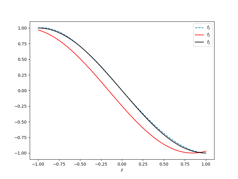
The approximation is close to the accuracy of \(f_{1, 2}\) without needing as many evaluations of \(f_{1}\)
Adaptivity
The the algorithm that adapts the sparse grid index set \(\mathcal{I}\) to the importance of each variable be modified for use with multi-index collocation [JEGG2019]. The algorithm is highly effective as it balances the interpolation error due to using a finite number of training points with the cost of evaluating the models of varying accuracy.
Lets build a multi-level sparse grid
import copy
from pyapprox.surrogates.interp.adaptive_sparse_grid import (
    plot_adaptive_sparse_grid_2d)
from pyapprox.util.visualization import get_meshgrid_function_data

config_values = [np.asarray([0.25, 0.125, 0])]
config_var_trans = ConfigureVariableTransformation(config_values)
mi_model = MultiIndexModel(setup_model, config_values)

#The sparse grid uses the wall time of the model execution as a cost function by default, but here we will use a custom cost function because all models are trivial to evaluate.

def cost_function(config_sample):
    canonical_config_sample = config_var_trans.map_to_canonical(
        config_sample)
    return (1+canonical_config_sample[0])**2

class AdaptiveCallback():
    def __init__(self, validation_samples, validation_values):
        self.validation_samples = validation_samples
        self.validation_values = validation_values

        self.nsamples = []
        self.errors = []
        self.sparse_grids = []

    def __call__(self, approx):
        self.nsamples.append(approx.samples.shape[1])
        approx_values = approx.evaluate_using_all_data(
            self.validation_samples)
        error = (np.linalg.norm(
            self.validation_values-approx_values) /
                     self.validation_samples.shape[1])
        self.errors.append(error)
        self.sparse_grids.append(copy.deepcopy(approx))


validation_samples = variable.rvs(100)
validation_values = mi_model._model_ensemble.functions[-1](validation_samples)
adaptive_callback = AdaptiveCallback(validation_samples, validation_values)
sg = adaptive_approximate(
    mi_model, variable, "sparse_grid",
    {"refinement_indicator": variance_refinement_indicator,
     "max_level_1d": [10,  len(config_values[0])-1],
     "univariate_quad_rule_info": None,
     "max_level": np.inf, "max_nsamples": 80,
     "config_variables_idx": nvars,
     "config_var_trans": config_var_trans,
     "cost_function": cost_function,
     "callback": adaptive_callback}).approx

from pyapprox.interface.wrappers import SingleFidelityWrapper
hf_model = SingleFidelityWrapper(mi_model, config_values[0][2:3])
mf_model = SingleFidelityWrapper(mi_model, config_values[0][1:2])
lf_model = SingleFidelityWrapper(mi_model, config_values[0][:1])
Now plot the adaptive algorithm
fig, axs = plt.subplots(1, 3, sharey=False, figsize=(3*8, 6))
plot_xx = np.linspace(-1, 1, 101)
def animate(ii):
    [ax.clear() for ax in axs]
    sg = adaptive_callback.sparse_grids[ii]
    plot_adaptive_sparse_grid_2d(sg, axs=axs[:2])
    axs[0].set_xlim([0, 10])
    axs[0].set_ylim([0, len(config_values[0])-1])
    axs[1].set_ylim([0, len(config_values[0])-1])
    axs[1].set_ylabel(r"$\alpha_1$")
    axs[2].plot(plot_xx, lf_model(plot_xx[None, :]), 'r', label=r"$f_0(z_1)$")
    axs[2].plot(plot_xx, mf_model(plot_xx[None, :]), 'g', label=r"$f_1(z_1)$")
    axs[2].plot(plot_xx, hf_model(plot_xx[None, :]), 'k', label=r"$f_2(z_1)$")
    axs[2].plot(plot_xx, sg(plot_xx[None, :]), '--b', label=r"$f_{I}(z_1)$")
    axs[2].set_xlabel(r"$z_1$")
    axs[2].legend(fontsize=18)


import matplotlib.animation as animation
ani = animation.FuncAnimation(
    fig, animate, interval=500,
    frames=len(adaptive_callback.sparse_grids), repeat_delay=1000)
ani.save("adaptive_misc.gif", dpi=100,
         writer=animation.ImageMagickFileWriter())
The lower fidelity models are evaluated more until they can no longer reduce the error in the sparse grid. At this point the interpolation error of the low-fidelity models is dominated by the bias in the exact low-fidelity models. Changing the cost_function will change how many samples are used to evaluate each model.
Three or more models
This tutorial only demonstrates the use of multi-level collocation with two models, but it can easily be used with three or more models. Try setting config_values = [np.asarray([0.25, 0.125, 0])]
Multi-index collocation
Multi-index collocation is an extension of mulit-level collocation that can be used with models that have multiple parameters controlling the numerical discretization, for example, the spatial and temporal resoutions of a finite element solver. While this tutorial does not demonstrate multi-index collocation it is supported by PyApprox.
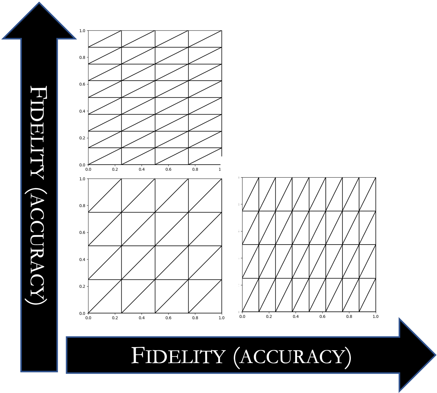
A multi-index hierarchy formed by increasing mesh discretizations in two different spatial directions. |
References
Total running time of the script: ( 0 minutes 12.479 seconds)