MFNets: Multi-fidelity networks

This tutorial describes how to implement and deploy multi-fidelity networks to construct a surrogate of the output of a high-fidelity model using a set of lower-fidelity models of lower accuracy and cost [GJGEIJUQ2020].

In the Multi-level and Multi-index Collocation tutorial we showed how multi-index collocation takes adavantage of a specific type of relationship between models to build a surrogate. In some applications this structure may not exist and so methods that can exploit other types of structures are needed. MFNets provide a means to encode problem specific relationships between information sources.

In the following we will approximate each information source with a linear subspace model. Specifically given a basis (features) ${\varphi }_{\alpha }=\{{\varphi }_{\alpha p}{\}}_{p=1}^P$ for each information source $\alpha =1\dots ,M$ we seek approximations of the form

$$Y_{\alpha }=h(Z_{\alpha }){\theta }_{\alpha }=\sum _{p=1}^{P_{\alpha }}{\varphi }_p(Z_{\alpha }){\theta }_{\alpha p}$$

Given data for each model $y_{\alpha }=[(y_{\alpha }^{(1)}{)}^{\mathrm{\top }},\dots ,(y_{\alpha }^{(N_{\alpha })}{)}^{\mathrm{\top }}{]}^{\mathrm{\top }}$ where $y_{\alpha }^{(i)}=h(z_{\alpha }^{(i)}){\theta }_{\alpha }+{ϵ}_{\alpha }^{(i)}\in {\mathbb{R}}^{1\times Q}$

MFNets provides a framework to encode correlation between information sources to with the goal of producing high-fidelity approximations which are more accurate than single-fidelity approximations using ony high-fidelity data. The first part of this tutorial will show how to apply MFNets to a simple problem using standard results for the posterior of Gaussian linear models. The second part of this tutorial will show how to generalize the MFNets procedure using Bayesian Networks.

Linear-Gaussian models

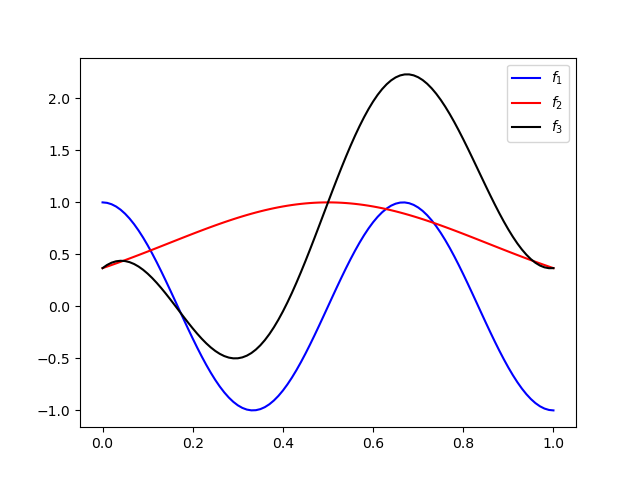
As our first example we will consider the following ensemble of three univariate information sources which are parameterized by the same variable $z_1$

$$\begin{array}{rl}{f}_1(z)& =\cos \left(3\pi z_1\right),\\ f_2(z)& =\exp (-0.5(z_1-0.5{)}^2),\\ f_3(z)& =f_1(z)+f_2(z)+2z_1-1\end{array}$$

Let’s first import the necessary functions and modules and set the seed for reproducibility

import networkx as nx
import numpy as np
import scipy
from scipy import stats
import matplotlib.pyplot as plt

from pyapprox.bayes.laplace import (
    laplace_posterior_approximation_for_linear_models)
from pyapprox.bayes.gaussian_network import (
    get_total_degree_polynomials, plot_1d_lvn_approx, GaussianNetwork,
    cond_prob_variable_elimination,
    convert_gaussian_from_canonical_form,
    plot_peer_network_with_data)

np.random.seed(2)

Now define the information sources and their inputs

nmodels = 3
def f1(x): return np.cos(3*np.pi*x).T
def f2(x): return np.exp(-(x-.5)**2/0.25).T
def f3(x): return f1(x)+f2(x)+(2*x-1).T


functions = [f1, f2, f3]
ensemble_univariate_variables = [[stats.uniform(0, 1)]]*nmodels

Plot the 3 functions

xx = np.linspace(0, 1, 101)[None, :]
plt.plot(xx[0, :],  f1(xx), label=r'$f_1$', c='b')
plt.plot(xx[0, :],  f2(xx), label=r'$f_2$', c='r')
plt.plot(xx[0, :],  f3(xx), label=r'$f_3$', c='k')
_ = plt.legend()

Now setup the polynomial approximations of each information source

degrees = [5]*nmodels
polys, nparams = get_total_degree_polynomials(
    ensemble_univariate_variables, degrees)

Next generate the training data. Here we will set the noise to be independent Gaussian with mean zero and variance ${0.01}^2$.

nsamples = [20, 20, 3]
samples_train = [p.var_trans.variable.rvs(n) for p, n in zip(polys, nsamples)]
noise_std = [0.01]*nmodels
noise = [noise_std[ii]*np.random.normal(
    0, noise_std[ii], (samples_train[ii].shape[1], 1)) for ii in range(nmodels)]
values_train = [f(s)+n for s, f, n in zip(samples_train, functions, noise)]

In the following we will assume a Gaussian prior on the coefficients of each approximation. Because the noise is also Gaussian and we are using linear subspace models the posterior of the approximation coefficients will also be Gaussian.

With the goal of applying classical formulas for the posterior of Gaussian-linear models let’s first define the linear model which involves all information sources

$$y=\mathrm{\Phi }\theta +ϵ$$

Specifically let ${\mathrm{\Phi }}_{\alpha }\in {\mathbb{R}}^{N_i\times P_i}$ be Vandermonde-like matrices with entries ${\varphi }_{\alpha p}(z_{\alpha }^{(n)})$ in the nth row and pth column. Now define $\mathrm{\Phi }=\mathrm{blockdiag}({\mathrm{\Phi }}_1,\dots ,{\mathrm{\Phi }}_M)$ and ${\mathrm{\Sigma }}_{ϵ}=\mathrm{blockdiag}({\mathrm{\Sigma }}_{ϵ1},\dots ,{\mathrm{\Sigma }}_{ϵM})$, $y={[y_1^{\mathrm{\top }},\dots ,y_M^{\mathrm{\top }}]}^{\mathrm{\top }}$, $\theta ={[{\theta }_1^{\mathrm{\top }},\dots ,{\theta }_M^{\mathrm{\top }}]}^{\mathrm{\top }}$, and $ϵ={[{ϵ}_1^{\mathrm{\top }},\dots ,{ϵ}_M^{\mathrm{\top }}]}^{\mathrm{\top }}$.

For our three model example we have

$$\begin{array}{r}\mathrm{\Phi }=\left[\begin{array}{ccc}{\mathrm{\Phi }}_1& 0_{N_1{P}_2}& 0_{N_1{P}_3}\\ 0_{N_2{P}_1}& {\mathrm{\Phi }}_2& 0_{N_2{P}_3}\\ 0_{N_3{P}_1}& 0_{N_3{P}_1}& {\mathrm{\Phi }}_3\end{array}\right]{\mathrm{\Sigma }}_{ϵ}=\left[\begin{array}{ccc}{\mathrm{\Sigma }}_{{ϵ}_1}& 0_{N_1{N}_2}& 0_{N_1{N}_3}\\ 0_{N_2{N}_1}& {\mathrm{\Sigma }}_{{ϵ}_2}& 0_{N_2{N}_3}\\ 0_{N_3{N}_1}& 0_{N_3{N}_1}& {\mathrm{\Sigma }}_{{ϵ}_3}\end{array}\right]y=\left[\begin{array}{c}{y}_1\\ y_2\\ y_3\end{array}\right]\end{array}$$

where the $0_{mp}\in {\mathbb{R}}^{m\times p}$ is a matrix of zeros.

basis_matrices = [p.basis_matrix(s) for p, s in zip(polys, samples_train)]
basis_mat = scipy.linalg.block_diag(*basis_matrices)
noise_matrices = [noise_std[ii]**2*np.eye(samples_train[ii].shape[1])
                  for ii in range(nmodels)]
noise_cov = scipy.linalg.block_diag(*noise_matrices)
values = np.vstack(values_train)

Now let the prior on the coefficients of $Y_{\alpha }$ be Gaussian with mean ${\mu }_{\alpha }$ and covariance ${\mathrm{\Sigma }}_{\alpha \alpha }$, and the covariance between the coefficients of different information sources $Y_{\alpha }$ and $Y_{\beta }$ be ${\mathrm{\Sigma }}_{\alpha \beta }$, such that the joint density of the coefficients of all information sources is Gaussian with mean and covariance given by

$$\begin{array}{r}\mu ={[{\mu }_1^{\mathrm{\top }},\dots ,{\mu }_M^{\mathrm{\top }}]}^{\mathrm{\top }}‘\mathrm{\Sigma }=\left[\begin{array}{cccc}{\mathrm{\Sigma }}_{11}& {\mathrm{\Sigma }}_{12}& \dots & {\mathrm{\Sigma }}_{1M}\\ {\mathrm{\Sigma }}_{21}& {\mathrm{\Sigma }}_{22}& \dots & {\mathrm{\Sigma }}_{2M}\\ ⋮& ⋮& \ddots & ⋮\\ {\mathrm{\Sigma }}_{M1}& {\mathrm{\Sigma }}_{M2}& \dots & {\mathrm{\Sigma }}_{MM}\end{array}\right]\end{array}$$

In the following we will set the prior mean to zero for all coefficients and first try setting all the coefficients to be independent

prior_mean = np.zeros((nparams.sum(), 1))
prior_cov = np.eye(nparams.sum())

With these definition the posterior distribution of the coefficients is (see Bayesian Inference)

$${\mathrm{\Sigma }}^{\mathrm{post}}={({\mathrm{\Sigma }}^{-1}+{\mathrm{\Phi }}^{\mathrm{\top }}{\mathrm{\Sigma }}_{ϵ}^{-1}\mathrm{\Phi })}^{-1},{\mu }^{\mathrm{post}}={\mathrm{\Sigma }}^{\mathrm{post}}({\mathrm{\Phi }}^{\mathrm{\top }}{\mathrm{\Sigma }}_{ϵ}^{-1}y+{\mathrm{\Sigma }}^{-1}\mu ),$$

post_mean, post_cov = laplace_posterior_approximation_for_linear_models(
    basis_mat, prior_mean, np.linalg.inv(prior_cov), np.linalg.inv(noise_cov),
    values)

Now let’s plot the resulting approximation of the high-fidelity data.

hf_prior = (prior_mean[nparams[:-1].sum():],
            prior_cov[nparams[:-1].sum():, nparams[:-1].sum():])
hf_posterior = (post_mean[nparams[:-1].sum():],
                post_cov[nparams[:-1].sum():, nparams[:-1].sum():])
xx = np.linspace(0, 1, 101)
fig, axs = plt.subplots(1, 1, figsize=(8, 6))
training_labels = [
    r'$f_1(z_1^{(i)})$', r'$f_2(z_2^{(i)})$', r'$f_3(z_2^{(i)})$']
plot_1d_lvn_approx(
    xx, nmodels, polys[2].basis_matrix, hf_posterior, hf_prior, axs,
    samples_train[2:], values_train[2:], training_labels[2:], [0, 1],
    colors=['k'], mean_label=r'$\mathrm{Single\;Fidelity}$')
axs.set_xlabel(r'$z$')
axs.set_ylabel(r'$f(z)$')
_ = plt.plot(xx, f3(xx), 'k', label=r'$f_3$')

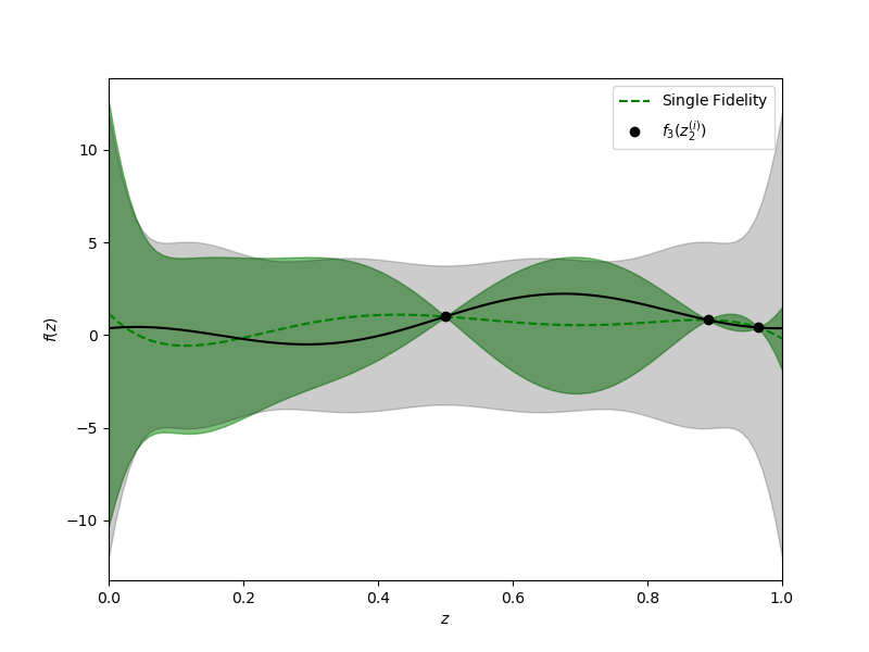
Unfortunately by assuming that the coefficients of each information source are independent the lower fidelity data is not informing the estimation of the coefficients of the high-fidelity approximation. This statement can be verified by computing an approximation with only the high-fidelity data

single_hf_posterior = laplace_posterior_approximation_for_linear_models(
    basis_matrices[-1], hf_prior[0], np.linalg.inv(hf_prior[1]),
    np.linalg.inv(noise_matrices[-1]), values_train[-1])
assert np.allclose(single_hf_posterior[0], hf_posterior[0])
assert np.allclose(single_hf_posterior[1], hf_posterior[1])

We can improve the high-fidelity approximation by encoding a correlation between the coefficients of each information source. In the following we will assume that the cofficients of an information source is linearly related to the coefficients of the other information sources. Specifically we will assume that

$${\theta }_{\alpha }=\sum _{\beta \in \mathrm{pa}(\alpha )}{A}_{\alpha \beta }{\theta }_{\beta }+b_{\alpha }+v_{\alpha },$$

where $b_{\alpha }\in {\mathbb{R}}^{P_{\alpha }}$ is a deterministic shift, $v_{\alpha }$ is a Gaussian noise with mean zero and covariance ${\mathrm{\Sigma }}_{v_{\alpha }}\in {\mathbb{R}}^{P_{\alpha }\times P_{\alpha }}$, and $\mathrm{pa}(\alpha )\subset \{\beta :\beta =1,\dots ,M,\beta \ne \alpha \}$ is a possibly empty subset of indices indexing the information sources upon which the $\alpha$ information source is dependent. Here $A_{\alpha \beta }\in {\mathbb{R}}^{P_{\alpha }\times P_{\beta }}$ are matrices which, along with ${\mathrm{\Sigma }}_{v\alpha }$, define the strength of the relationship between the coefficients of each information source. When these matrices are dense each coefficient of $Y_{\alpha }$ is a function of all coefficients in $Y_{\beta }$. It is often more appropriate, however to impose a sparse structure. For example if $A$ is diagonal this implies that the coefficient of a certain basis in the representation of one information source is only related to the coefficient of the same basis in the other information sources.

Note this notation comes from the literature on Bayesian networks which we will use in the next section to generalize the procedure described in this tutorial to large ensembles of information sources with complex dependencies.

The variable $v_{\alpha }$ is a random variable that controls the correlation between the coefficients of the information sources. The MFNets framework in [GJGEIJUQ2020] assumes that this variable is Gaussian with mean zero and covariance given by ${\mathrm{\Sigma }}_{v\alpha }$. In this example we will set

$${\theta }_3=A_{31}{\theta }_1+A_{32}{\theta }_2+b_3+v_3$$

and assume that $\mathbb{C}\text{ov}[{\theta }_{\alpha },v_3]=0\mathrm{\forall }\alpha$ and $\mathbb{C}\text{ov}[{\theta }_1,{\theta }_2]=0$. Note the later relationship does not mean data from the information from $Y_1$ cannot be used to inform the coefficients of $Y_2$.

Given the defined relationship between the coefficients of each information source we can compute the prior over the joint distribiution of the coefficients of all information sources. Without loss of generality we assume the variables have zero mean and $b_3=0$ so that

$$\mathbb{C}\text{ov}[{\theta }_1,{\theta }_3]=\mathbb{E}\left[{\theta }_1{\theta }_3^{\mathrm{\top }}\right]=\mathbb{E}\left[{\theta }_1{(A_{31}{\theta }_1+A_{32}{\theta }_2+v_{\alpha })}^{\mathrm{\top }}\right]=\mathbb{C}\text{ov}[{\theta }_1,{\theta }_1]A_{31}^{\mathrm{\top }}$$

similarly $\mathbb{C}\text{ov}[{\theta }_2,{\theta }_3]=\mathbb{C}\text{ov}[{\theta }_2,{\theta }_2]A_{32}^{\mathrm{\top }}$. We also have

$$\begin{array}{rl}\mathbb{C}\text{ov}[{\theta }_3,{\theta }_3]& =\mathbb{E}\left[{\theta }_1{\theta }_1^{\mathrm{\top }}\right]=\mathbb{E}\left[(A_{13}{\theta }_1+A_{12}{\theta }_2+v_{\alpha }){(A_{31}{\theta }_1+A_{32}{\theta }_2+v_3)}^{\mathrm{\top }}\right]\\ & =A_{31}\mathbb{C}\text{ov}[{\theta }_1,{\theta }_1]A_{31}^{\mathrm{\top }}+A_{32}\mathbb{C}\text{ov}[{\theta }_2,{\theta }_2]A_{32}^{\mathrm{\top }}+\mathbb{C}\text{ov}[v_3,v_3]\end{array}$$

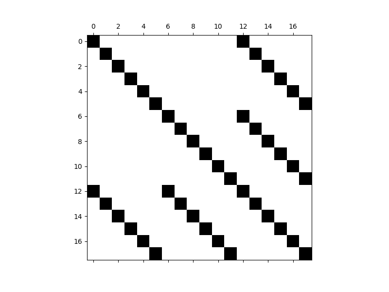
In this tutorial we will set $A_{31}=a_{31}I$, $A_{32}=a_{32}I$, ${\mathrm{\Sigma }}_{11}=s_{11}I$, ${\mathrm{\Sigma }}_{22}=s_{22}I$ and ${\mathrm{\Sigma }}_{v_3}=v_{3}I$ to be diagonal matrices with the same value for all entries on the diagonal which gives

$$\begin{array}{r}\mathrm{\Sigma }=\left[\begin{array}{ccc}{\mathrm{\Sigma }}_{11}& 0& a_{31}{\mathrm{\Sigma }}_{11}\\ 0& {\mathrm{\Sigma }}_{22}& a_{32}{\mathrm{\Sigma }}_{22}\\ a_{31}{\mathrm{\Sigma }}_{11}& a_{32}{\mathrm{\Sigma }}_{22}& a_{31}^2{\mathrm{\Sigma }}_{11}+a_{32}^2{\mathrm{\Sigma }}_{22}+{\mathrm{\Sigma }}_{v_3}\end{array}\right]\end{array}$$

In the following we want to set the prior covariance of each individual information source to be the same, i.e. we set $s_{11}=s_{22}$ and $v_3=s_{33}-(a_{31}^2{\mathrm{\Sigma }}_{11}+a_{32}^2{\mathrm{\Sigma }}_{22})$

I1, I2, I3 = np.eye(degrees[0]+1), np.eye(degrees[1]+1), np.eye(degrees[2]+1)

s11, s22, s33 = [1]*nmodels
a31, a32 = [0.7]*(nmodels-1)
#if a31==32 and s11=s22=s33=1 then a31<=1/np.sqrt(2))
assert (s33-a31**2*s11-a32**2*s22) > 0
rows = [np.hstack([s11*I1, 0*I1, a31*s11*I1]),
        np.hstack([0*I2, s22*I2, a32*s22*I2]),
        np.hstack([a31*s11*I3, a32*s22*I3, s33*I3])]
prior_cov = np.vstack(rows)

Plot the structure of the prior covariance

fig, axs = plt.subplots(1, 1, figsize=(8, 6))
_ = plt.spy(prior_cov)

post_mean, post_cov = laplace_posterior_approximation_for_linear_models(
    basis_mat, prior_mean, np.linalg.inv(prior_cov), np.linalg.inv(noise_cov),
    values)

Now let’s plot the resulting approximation of the high-fidelity data.

hf_prior = (prior_mean[nparams[:-1].sum():],
            prior_cov[nparams[:-1].sum():, nparams[:-1].sum():])
hf_posterior = (post_mean[nparams[:-1].sum():],
                post_cov[nparams[:-1].sum():, nparams[:-1].sum():])
xx = np.linspace(0, 1, 101)
fig, axs = plt.subplots(1, 1, figsize=(8, 6))
training_labels = [
    r'$f_1(z_1^{(i)})$', r'$f_2(z_2^{(i)})$', r'$f_3(z_2^{(i)})$']
plot_1d_lvn_approx(xx, nmodels, polys[2].basis_matrix, hf_posterior, hf_prior,
                   axs, samples_train, values_train, training_labels, [0, 1],
                   colors=['b', 'r', 'k'])
axs.set_xlabel(r'$z$')
axs.set_ylabel(r'$f(z)$')
_ = plt.plot(xx, f3(xx), 'k', label=r'$f_3$')

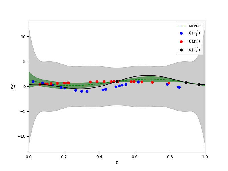
Depsite using only a very small number of samples of the high-fidelity information source, the multi-fidelity approximation has smaller variance and the mean more closely approximates the true high-fidelity information source, when compared to the single fidelity strategy.

Gaussian Networks

In this section of the tutorial we will use show how to use Gaussian (Bayesian networks to encode a large class of relationships between information sources and perform compuationally efficient inference. This tutorial builds on the material presented in the Gaussian Networks tutorial.

In the following we will use use Gaussian networks to fuse information from a modification of the information enembles used in the previous section. Specifically consider the enemble

$$\begin{array}{rl}{f}_1(z)& =\cos (3\pi z_1+0.1z_2),\\ f_2(z)& =\exp (-0.5(z_1-0.5{)}^2),\\ f_3(z)& =f_2(z)+\cos (3\pi z_1)\end{array}$$

nmodels = 3
def f1(x): return np.cos(3*np.pi*x[0, :]+0.1*x[1, :])[:, np.newaxis]
def f2(x): return np.exp(-(x-.5)**2/0.5).T
def f3(x): return f2(x)+np.cos(3*np.pi*x).T


functions = [f1, f2, f3]

ensemble_univariate_variables = [
    [stats.uniform(0, 1)]*2]+[[stats.uniform(0, 1)]]*2

The difference between this example and the previous is that one of the low-fidelity information sources has two inputs in contrast to the other sources (functions) which have one. These types of sources CANNOT be fused by other multi-fidelity methods. Fusion is possible with MFNets because it relates information sources through correlation between the coefficients of the approximations of each information source. In the context of Bayesian networks the coefficients are called latent variables.

Again assume that the coefficients of one source are only related to the coefficient of the corresponding basis function in the parent sources. Note that unlike before the $A_{ij}$ matrices will not be diagonal. The polynomials have different numbers of terms and so the $A_{ij}$ matrices will be rectangular. They are essentially a diagonal matrix concatenated with a matrix of zeros. Let $A_{31}^{\mathrm{nz}}=a_{31}I\in {\mathbb{R}}^{P_1\times P_1}$ be a diagonal matrix relating the coefficients of all the shared terms in $Y_1,Y_3$. Then $A_{31}^{\mathrm{nz}}=[A_{31}^{\mathrm{nz}}{0}_{P_3\times (P_1-P_3)}]\in {\mathbb{R}}^{P_1\times P_2}$.

Use the following to setup a Gaussian network for our example

degrees = [3, 5, 5]
polys, nparams = get_total_degree_polynomials(
    ensemble_univariate_variables, degrees)
basis_matrix_funcs = [p.basis_matrix for p in polys]

s11, s22, s33 = [1]*nmodels
a31, a32 = [0.7]*(nmodels-1)
cpd_scales = [a31, a32]
prior_covs = [s11, s22, s33]

nnodes = 3
graph = nx.DiGraph()
prior_covs = [1, 1, 1]
prior_means = [0, 0, 0]
cpd_scales = [a31, a32]
node_labels = [f'Node_{ii}' for ii in range(nnodes)]
cpd_mats = [None, None,
            np.hstack([cpd_scales[0]*np.eye(nparams[2], nparams[0]),
                       cpd_scales[1]*np.eye(nparams[2], nparams[1])])]

for ii in range(nnodes-1):
    graph.add_node(
        ii, label=node_labels[ii],
        cpd_cov=prior_covs[ii]*np.eye(nparams[ii]),
        nparams=nparams[ii], cpd_mat=cpd_mats[ii],
        cpd_mean=prior_means[ii]*np.ones((nparams[ii], 1)))
#WARNING Nodes have to be added in order their information appears in lists.
#i.e. high-fidelity node must be added last.
ii = nnodes-1
cov = np.eye(nparams[ii])*(prior_covs[ii]-np.dot(
    np.asarray(cpd_scales)**2, prior_covs[:ii]))
graph.add_node(
    ii, label=node_labels[ii], cpd_cov=cov, nparams=nparams[ii],
    cpd_mat=cpd_mats[ii],
    cpd_mean=(prior_means[ii]-np.dot(cpd_scales[:ii], prior_means[:ii])) *
    np.ones((nparams[ii], 1)))


graph.add_edges_from([(ii, nnodes-1) for ii in range(nnodes-1)])


network = GaussianNetwork(graph)

We can compute the prior from this network using by instantiating the factors used to represent the joint density of the coefficients and then multiplying them together using the conditional probability variable elimination algorithm. We will describe this algorithm in more detail when infering the posterior distribution of the coefficients from data using the graph. When computing the prior this algorithm simply amounts to multiplying the factors of the graph together.

network.convert_to_compact_factors()
labels = [l[1] for l in network.graph.nodes.data('label')]
factor_prior = cond_prob_variable_elimination(
    network, labels)
prior = convert_gaussian_from_canonical_form(
    factor_prior.precision_matrix, factor_prior.shift)
#print('Prior covariance',prior[1])

#To infer the uncertain coefficients we must add training data to the network.
nsamples = [10, 10, 2]
samples_train = [p.var_trans.variable.rvs(n) for p, n in zip(polys, nsamples)]
noise_std = [0.01]*nmodels
noise = [noise_std[ii]*np.random.normal(
    0, noise_std[ii], (samples_train[ii].shape[1], 1)) for ii in range(nmodels)]
values_train = [f(s)+n for s, f, n in zip(samples_train, functions, noise)]

data_cpd_mats = [
    b(s) for b, s in zip(basis_matrix_funcs, samples_train)]
data_cpd_vecs = [np.zeros(nsamples[ii]) for ii in range(nmodels)]
noise_covs = [np.eye(nsamples[ii])*noise_std[ii]**2
              for ii in range(nnodes)]

network.add_data_to_network(data_cpd_mats, data_cpd_vecs, noise_covs)
fig, ax = plt.subplots(1, 1, figsize=(8, 5))
_ = plot_peer_network_with_data(network.graph, ax)

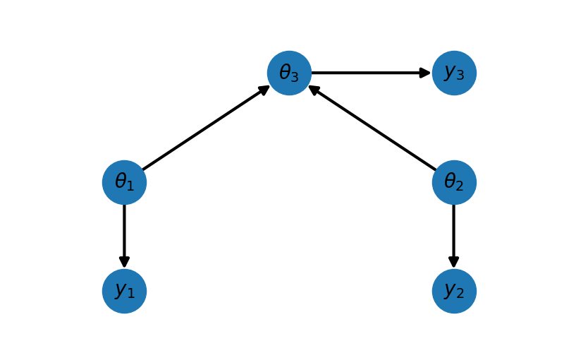
For this network we have $\mathrm{pa}(1)=\mathrm{\varnothing },\mathrm{pa}(1)=\mathrm{\varnothing },\mathrm{pa}(2)=\{1,2\}$ and the graph has one CPDs which for this example is given by

$$\mathbb{P}({\theta }_3\mid {\theta }_1,{\theta }_2)\sim \mathcal{N}(A_{31}{\theta }_1+A_{32}{\theta }_2+b_3,{\mathrm{\Sigma }}_{v_3}),$$

with $b_3=0$.

We refer to a Gaussian network based upon this DAG as a peer network. Consider the case where a high fidelity simulation model incorporates two sets of active physics, and the two low-fidelity peer models each contain one of these components. If the high-fidelity model is given, then the low-fidelity models are no longer independent of one another. In other words, information about the parameters used in one set of physics will inform the other set of physics because they are coupled together in a known way through the high-fidelity model.

The joint density of the network is given by

$$\mathbb{P}({\theta }_1,{\theta }_2,{\theta }_3)=\mathbb{P}({\theta }_3\mid {\theta }_1,{\theta }_2)\mathbb{P}({\theta }_1)\mathbb{P}({\theta }_2)$$

#convert_to_compact_factors must be after add_data when doing inference
network.convert_to_compact_factors()
labels = ['Node_2']
evidence, evidence_ids = network.assemble_evidence(values_train)
factor_post = cond_prob_variable_elimination(
    network, labels, evidence_ids=evidence_ids, evidence=evidence)
hf_posterior = convert_gaussian_from_canonical_form(
    factor_post.precision_matrix, factor_post.shift)
factor_prior = cond_prob_variable_elimination(
    network, labels)
hf_prior = convert_gaussian_from_canonical_form(
    factor_prior.precision_matrix, factor_prior.shift)

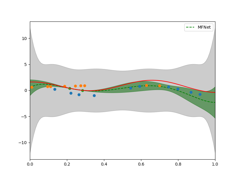
xx = np.linspace(0, 1, 101)
fig, axs = plt.subplots(1, 1, figsize=(8, 6))
plot_1d_lvn_approx(xx, nmodels, polys[2].basis_matrix, hf_posterior, hf_prior,
                   axs, samples_train, values_train, None, [0, 1])
_ = axs.plot(xx, functions[2](xx[np.newaxis, :]), 'r', label=r'$f_3$')

References

[GJGEIJUQ2020] (1,2)

A. Gorodetsky et al. MFNets: Multi-fidelity data-driven networks for bayesian learning and prediction, International Journal for Uncertainty Quantification, 2020.

Appendix

There is a strong connection between the mean of the Bayes posterior distribution of linear-Gaussian models with least squares regression. Specifically the mean of the posterior is equivalent to linear least-squares regression with a regulrization that penalizes deviations from the prior estimate of the parameters. Let the least squares objective function be

$$f(\theta )=\frac{1}{2}(y-A\theta {)}^{\mathrm{\top }}{\mathrm{\Sigma }}_{ϵ}^{-1}(y-A\theta )+\frac{1}{2}({\mu }_{\theta }-\theta {)}^{\mathrm{\top }}{\mathrm{\Sigma }}_{\theta }^{-1}({\mu }_{\theta }-\theta ),$$

where the first term on the right hand side is the usual least squares objective and the second is the regularization term. This regularized objective is minimized by setting its gradient to zero, i.e.

$${\mathrm{\nabla }}_{\theta }f(\theta )=A^{\mathrm{\top }}{\mathrm{\Sigma }}_{ϵ}^{-1}(y-A\theta )+{\mathrm{\Sigma }}_{\theta }^{-1}({\mu }_{\theta }-\theta )=0,$$

thus

$$A^{\mathrm{\top }}{\mathrm{\Sigma }}_{ϵ}^{-1}A\theta +{\mathrm{\Sigma }}_{\theta }^{-1}\theta =A^{\mathrm{\top }}{\mathrm{\Sigma }}_{ϵ}^{-1}y+{\mathrm{\Sigma }}_{\theta }^{-1}{\mu }_{\theta }$$

and so

$$\theta ={(A^{\mathrm{\top }}{\mathrm{\Sigma }}_{ϵ}^{-1}A\theta +{\mathrm{\Sigma }}_{\theta }^{-1})}^{-1}(A^{\mathrm{\top }}{\mathrm{\Sigma }}_{ϵ}^{-1}y+{\mathrm{\Sigma }}_{\theta }^{-1}{\mu }_{\theta }).$$

Noting that ${(A^{\mathrm{\top }}{\mathrm{\Sigma }}_{ϵ}^{-1}A\theta +{\mathrm{\Sigma }}_{\theta }^{-1})}^{-1}$ is the posterior covariance we obtain the usual expression for the posterior mean

$${\mu }^{\mathrm{post}}={\mathrm{\Sigma }}^{\mathrm{post}}(A^{\mathrm{\top }}{\mathrm{\Sigma }}_{ϵ}^{-1}y+{\mathrm{\Sigma }}_{\theta }^{-1}{\mu }_{\theta })$$