Multilevel Best Linear Unbiased estimators (MLBLUE)

This tutorial introduces Multilevel Best Linear Unbiased estimators (MLBLUE) [SUSIAMUQ2020], [SUSIAMUQ2021] and compares its characteristics and performance with the previously introduced multi-fidelity estimators.

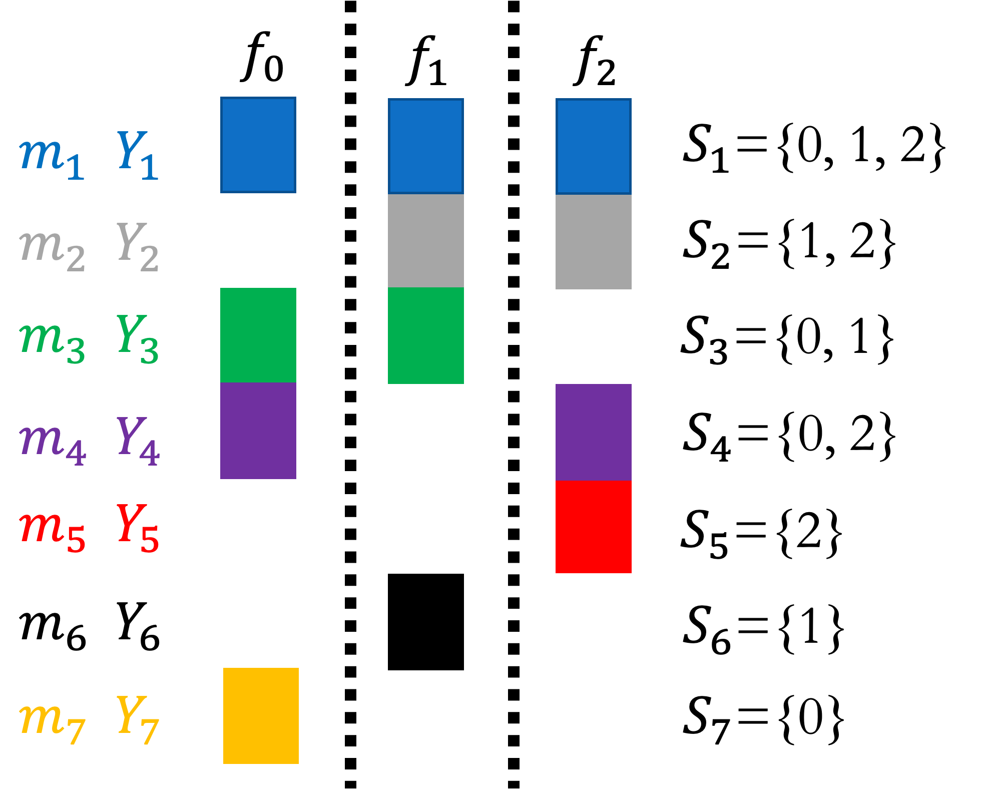
MLBLUE sample allocations.

MLBLUE assumes that each model \(f_1,\ldots,f_M\) is linearly dependent on the means of each model \(q=[Q_1,\ldots,Q_M]^\top\), where \(M\) is the number of low-fidelity models. Specifically, MLBLUE assumes that

\[Y=Hq+\epsilon,\]

where \(Y=[Y_1,\ldots,Y_{K}]\) are evaluations of models within all \(K=2^{M}-1\) nonempty subset \(S^k\in2^{\{1,\ldots,M\}}\setminus\emptyset\) , that is \(Y_k=[f_{S_k, 1}^{(1)},\ldots,f_{S_k, |S_k|}^{(1)},\ldots,f_{S_k, 1}^{(m_k)},\ldots,f_{S_k, |S_k|}^{(m_k)}]\). An example of such sets is shown in the figure above where \(m_k\) denotes the number of samples of each model in the subset \(S_k\).

Here \(H\) is a restriction opeator that specifies the means that produce the data in each set, that is

\[H=[R_1^\top,\ldots,R_K^\top]^\top, \qquad R_kq = [Q_{S_k,1},\ldots,Q_{S_k,|S_k|}]^\top\]

MLBLUE then finds the means of all models bys solving the generalized least squares problem

\[\min_{q\in\reals^M} \lVert Y-Hq\rVert^2_{{\covar{\epsilon}{\epsilon}}^{-1}}\]

Here ${covar{epsilon}{epsilon}$ is a matrix that is dependent on the covariance between the models and is given by

\[\begin{split}\covar{\epsilon}{\epsilon}&=\mathrm{BlockDiag}(G_1,\ldots, G_K),\quad G_k = \mathrm{BlockDiag}((C_k)_{i=1}^{m_k}), \\ C_k &= \covar{Y-H_kq}{Y-H_kq}.\end{split}\]

The figure below gives an example of the construction of the least squares system when only three subsets are active, \(S_2, S_3, S_5\); one, one and two samples of the models in each subset are taken, respectively. \(S_2\) only contributes on equation because it consists one model that is only sampled once. \(S_3\) contributes two equations, because it consists of two models sampled once each. Finally, \(S_5\) contributes four equations because it consists of two models sampled twice.

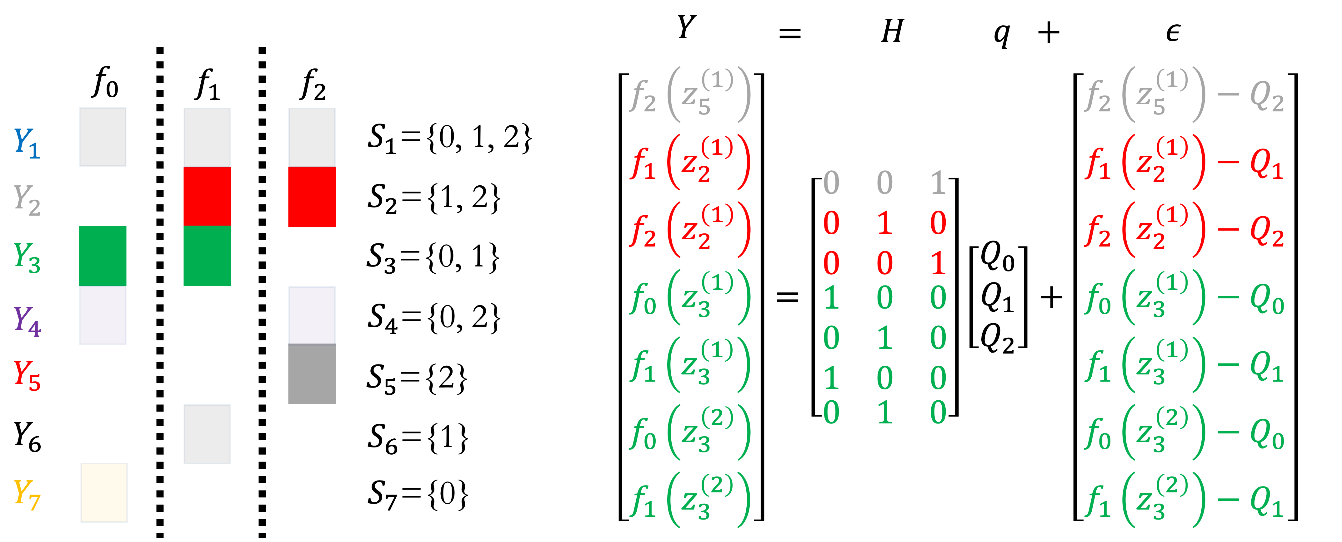
Example of subset data construction.

The figure below depicts the structure of the \(\covar{\epsilon}{\epsilon}\) for the same example, where \(\sigma_{ij}^2\) denotes the covariance between the models \(f_i,f_j\) and must be computed from a pilot study.

Example of the covariance structure.

The solution to the generalized least-squares problem can be found by solving the sustem of linear equations

\[\Psi q^B=y,\]

where q^B denotes the MLBLUE estimate of the model means \(q\) and

\[\Psi = \sum_{k=1}^K m_k R_k^\top C_k^{-1} R_k, \qquad y = \sum_{k=1}^K R^\top_K C_k^{-1} \sum_{i=1}^{m_k} Y_{k}^{(i)}\]

The vector \(q^B\) is an estimate of all model means, however one is often only interested in a linear combination of means, i.e.

\[q^B_\beta = \beta^\top q^B.\]

For example, \(\beta=[1, 0, \ldots, 0]^\top\) can be used to estimate only the high-fidelity mean.

Given $beta$ the variance of the MLBLU estimator is

\[\var{Q^B_\beta}=\beta^\top\Psi^{-1}\beta\]

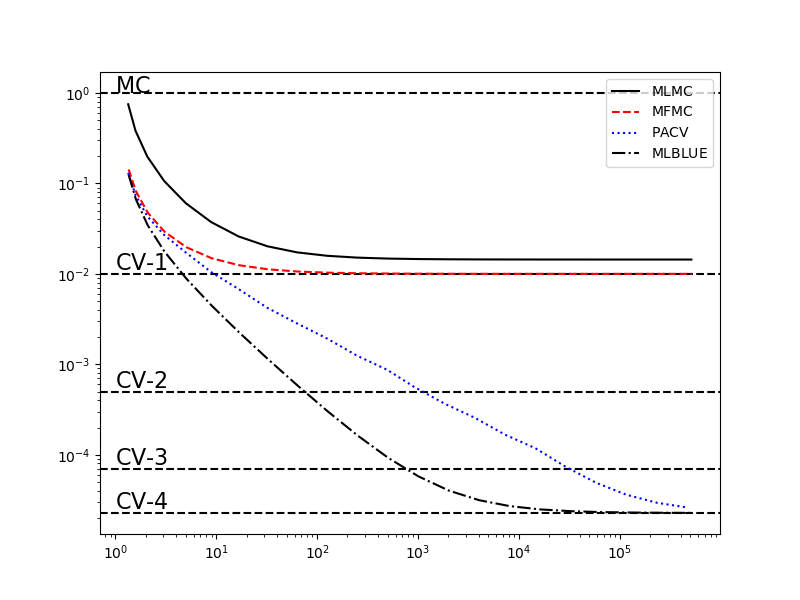
The following code compares MLBLUE to other multif-fidelity esimators when the number of high-fidelity samples is fixed and the number of low-fidelity samples increases. This example shows that unlike MLMC and MFMC, MLBLUE like ACV obtains the optimal variance reduction obtained by control variate MC, using known means, as the number of low-fidelity samples becomes very large.

First setup the polynomial benchmark

import numpy as np
import matplotlib.pyplot as plt

from pyapprox.util.visualization import mathrm_labels
from pyapprox.benchmarks import setup_benchmark
from pyapprox.multifidelity.factory import (
    get_estimator, compare_estimator_variances, compute_variance_reductions,
    multioutput_stats)
from pyapprox.multifidelity.visualize import (
    plot_estimator_variance_reductions)

First, plot the variance reduction of the optimal control variates using known low-fidelity means.

Second, plot the variance reduction of multi-fidelity estimators that do not assume known low-fidelity means. The code below repeatedly doubles the number of low-fidelity samples according to the initial allocation defined by nsample_ratios_base=[2,4,8,16].

benchmark = setup_benchmark("polynomial_ensemble")
model = benchmark.fun

nmodels = 5
cov = benchmark.covariance
costs = np.asarray([10**-ii for ii in range(nmodels)])
nhf_samples = 1

cv_stats, cv_ests = [], []
for ii in range(1, nmodels):
    cv_stats.append(multioutput_stats["mean"](benchmark.nqoi))
    cv_stats[ii-1].set_pilot_quantities(cov[:ii+1, :ii+1])
    cv_ests.append(get_estimator(
        "cv", cv_stats[ii-1], costs[:ii+1],
        lowfi_stats=benchmark.mean[1:ii+1]))
cv_labels = mathrm_labels(["CV-{%d}" % ii for ii in range(1, nmodels)])
target_cost = nhf_samples*sum(costs)
[est.allocate_samples(target_cost) for est in cv_ests]
cv_variance_reductions = compute_variance_reductions(cv_ests)[0]

from util import (
    plot_control_variate_variance_ratios,
    plot_estimator_variance_ratios_for_polynomial_ensemble)

estimators = [
    get_estimator("mlmc", cv_stats[-1], costs),
    get_estimator("mfmc", cv_stats[-1], costs),
    get_estimator("grd", cv_stats[-1], costs, tree_depth=4),
    get_estimator("mlblue", cv_stats[-1], costs, subsets=[
        np.array([0, 1, 2, 3, 4]),  np.array([1, 2, 3, 4]),
        np.array([2, 3, 4]), np.array([3, 4]), np.array([4,])])]
est_labels = est_labels = mathrm_labels(["MLMC", "MFMC", "PACV", "MLBLUE"])

ax = plt.subplots(1, 1, figsize=(8, 6))[1]
plot_control_variate_variance_ratios(cv_variance_reductions, cv_labels, ax)
_ = plot_estimator_variance_ratios_for_polynomial_ensemble(
    estimators, est_labels, ax)

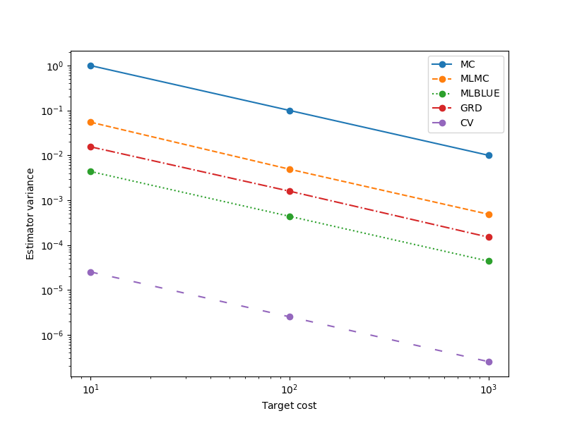
Optimal sample allocation

In the following we show how to optimize the sample allocation of MLBLUE and compare the optimized estimator to other alternatives.

The optimal sample allocation is obtained by solving

\[\min_{m\in\mathbb{N}_0^K}\var{Q^B_\beta(m)}\quad\text{such that}\quad\sum_{k=1}^K m_k \sum_{j=1}^{|S_k|} W_j \le W_{\max},\]

where \(W_j\) denotes the cost of evaluating the jth model and \(W_{\max}\) is the total budget.

This optimization problem can be solved effectively using semi-definite programming [CWARXIV2023].

target_costs = np.array([1e1, 1e2, 1e3], dtype=int)
estimators = [
    get_estimator("mc", cv_stats[-1], costs),
    get_estimator("mlmc", cv_stats[-1], costs),
    get_estimator("mlblue", cv_stats[-1], costs, subsets=[
        np.array([0, 1, 2, 3, 4]),  np.array([1, 2, 3, 4]),
        np.array([2, 3, 4]), np.array([3, 4]), np.array([4,])]),
    get_estimator("gmf", cv_stats[-1], costs, tree_depth=4),
    get_estimator("cv", cv_stats[-1], costs,
                  lowfi_stats=benchmark.mean[1:])]
est_labels = mathrm_labels(["MC", "MLMC", "MLBLUE", "GRD", "CV"])
optimized_estimators = compare_estimator_variances(
    target_costs, estimators)

from pyapprox.multifidelity.visualize import (
    plot_estimator_variances, plot_estimator_sample_allocation_comparison)
fig, axs = plt.subplots(1, 1, figsize=(1*8, 6))
_ = plot_estimator_variances(
    optimized_estimators, est_labels, axs,
    relative_id=0, cost_normalization=1)

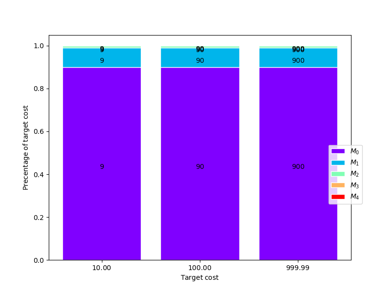
Now plot the number of samples allocated for each target cost

model_labels = [r"$M_{0}$".format(ii) for ii in range(cov.shape[0])]
fig, axs = plt.subplots(1, 1, figsize=(1*8, 6))
_= plot_estimator_sample_allocation_comparison(
    optimized_estimators[-1], model_labels, axs)

References

[SUSIAMUQ2020]

D. Schaden, E. Ullmann. On multilevel best linear unbiased estimators, SIAM/ASA J. Uncertainty Quantification 8 (2): 601 - 635, 2020.

[SUSIAMUQ2021]

D. Schaden, E. Ullmann. Asymptotic Analysis of Multilevel Best Linear Unbiased Estimators. SIAM/ASA Journal on Uncertainty Quantification 9 (3):953-978, 2021.

[CWARXIV2023]

M. Croci, K. Willcox, S. Wright. Multi-output multilevel best linear unbiased estimators via semidefinite programming. (2023)