Multi-level Monte Carlo

This tutorial builds upon Two model Approximate Control Variate Monte Carlo and describes how the pioneering work of Multi-level Monte Carlo (MLMC) [CGSTCVS2011], [GOR2008] can be used to estimate the mean of a high-fidelity model using multiple low fidelity models. MLMC is actually a special type of ACV estimator, but it was not originally derived this way. Consequently, this tutorial begins by presenting the typical formulation of MLMC and then concludes by discussing relationships with ACV.

Two Model MLMC

The two model MLMC estimator is based upon the observations that we can estimate

\[\mean{f_0}=\mean{f_1}+\mean{f_0-f_1}\]

using the following unbiased estimator

\[Q_{0}^\mathrm{ML}(\rvset_0,\rvset_1)=N_1^{-1}\sum_{i=1}^{N_1} f_{1}^{(i)}(\rvset_1)+N_0^{-1}\sum_{i=1}^{N_0} \left(f_{0}^{(i)}(\rvset_0)-f_{1}^{(i)}(\rvset_0)\right),\]

where \(f_{\alpha}^{(i)}(\rvset_\kappa)\) denotes an evaluation of \(f_\alpha\) using a sample from the set \(\rvset_\kappa\). To evaluate this estimator we must evaluate the low fidelity model at a set of samples \(\rvset_1\) and then evaluate the difference between the two models at another independet set \(\rvset_0\).

To simplify notation let

\[Y_{\alpha}(\rvset_{\alpha})=-N_{\alpha}^{-1}\sum_{i=1}^{N_{\alpha}} \left(f_{\alpha+1}^{(i)}(\rvset_{\alpha})-f_{\alpha}^{(i)}(\rvset_{\alpha})\right)\]

so we can write

\[Q_{0}^\mathrm{ML}(\rvset_0,\rvset_1)=Y_{0}(\rvset_0)+Y_{1}(\rvset_1)\]

where \(f_{2}=0\).

Now it is easy to see that the variance of this estimator is given by

\[\var{Q_{0}^\mathrm{ML}(\rvset_0, \rvset_1)}=\var{Y_{0}(\rvset_0)+Y_{1}(\rvset_1)}=N_0^{-1}\var{Y_{0}(\rvset_0)}+N_1^{-1}\var{Y_{1}(\rvset_1)}\]

where \(N_\alpha = |\rvset_\alpha|\) and we used the fact

\(\rvset_0\bigcap\rvset_1=\emptyset\) so \(\covar{Y_{0}(\rvset_0)}{Y_{0}(\rvset_1)}=0\)

From the previous equation we can see that MLMC works well if the variance of the difference between models is smaller than the variance of either model. Although the variance of the low-fidelity model is likely high, we can set \(N_0\) to be large because the cost of evaluating the low-fidelity model is low. If the variance of the discrepancy is smaller we only need a smaller number of samples so that the two sources of error (the two terms on the RHS of the previous equation) are balanced.

Note above and below we assume that \(f_0\) is the high-fidelity model, but typical multi-level literature assumes \(f_M\) is the high-fidelity model. We adopt the reverse ordering to be consistent with control variate estimator literature.

Many Model MLMC

MLMC can easily be extended to estimator based on \(M+1\) models. Letting \(f_0,\ldots,f_M\) be an ensemble of \(M+1\) models ordered by decreasing fidelity and cost (note typically MLMC literature reverses this order), we simply introduce estimates of the differences between the remaining models. That is

(1)\[Q_{0}^\mathrm{ML}(\rvset) = \sum_{\alpha=0}^M Y_{\alpha}(\rvset_\alpha), \quad f_{M+1}=0\]

To compute this estimator we use the following algorithm, starting with \(\alpha=M\)

1. Draw \(N_\alpha\) samples randomly from the PDF \(\pdf\) of the random variables.

2. Estimate \(f_{\alpha}\) and \(f_{\alpha}\) at the samples \(\rvset_\alpha\)

3. Compute the discrepancies \(Y_{\alpha,\rvset_\alpha}\) at each sample.

4. Decrease \(\alpha\) and repeat steps 1-3. until \(\alpha=0\).

5. Compute the ML estimator using (1)

In the above algorithm, we evaluate only the lowest fidelity model with \(\rvset_M\) (this follows from the assumption that \(f_{M+1}=0\)) and evaluate each discrepancies between each pair of consecutive models at the sets \(\rvset_\alpha\), such that \(\rvset_\alpha\cap\rvset_\beta=\emptyset,\; \alpha\neq\beta\) and the variance of the MLMC estimator is

\[\var{Q_{0}^\mathrm{ML}(\rvset_0, \ldots, \rvset_M)} = \sum_{\alpha=0}^M N_\alpha\var{Y_{\alpha}(\rvset_\alpha)}\]

Optimal Sample Allocation

When estimating the mean, the optimal allocation can be determined analytically. The following follows closely the exposition in [GAN2015] to derive the optimal allocation.

Let \(C_\alpha\) be the cost of evaluating the function \(f_\alpha\) at a single sample, then the total cost of the MLMC estimator is

\[C_{\mathrm{tot}}=\sum_{\alpha=0}^M C_\alpha N_\alpha\]

Now recall that the variance of the estimator is

\[\var{Q_0^\mathrm{ML}}=\sum_{\alpha=0}^M \var{Y_\alpha}N_\alpha,\]

where \(Y_\alpha\) is the disrepancy between two consecutive models, e.g. \(f_{\alpha-1}-f_\alpha\) and \(N_\alpha\) be the number of samples allocated to resolving the discrepancy, i.e. \(N_\alpha=\lvert\hat{\rvset}_\alpha\rvert\). Then For a fixed variance \(\epsilon^2\) the cost of the MLMC estimator can be minimized, by solving

\[\begin{split}\min_{N_0,\ldots,N_M} & \sum_{\alpha=0}^M\left(N_\alpha C_\alpha\right)\\ \mathrm{subject}\; \mathrm{to} &\sum_{\alpha=0}^M\left(N_\alpha^{-1}\var{Y_\alpha}\right)=\epsilon^2\end{split}\]

or alternatively by introducing the lagrange multiplier \(\lambda^2\) we can minimize

\[\begin{split}\mathcal{J}(N_0,\ldots,N_M,\lambda)&=\sum_{\alpha=0}^M\left(N_\alpha C_\alpha\right)+\lambda^2\left(\sum_{\alpha=0}^M\left(N_\alpha^{-1}\var{Y_\alpha}\right)-\epsilon^2\right)\\ &=\sum_{\alpha=0}^M\left(N_\alpha C_\alpha+\lambda^2N_\alpha^{-1}\var{Y_\alpha}\right)-\lambda^2\epsilon^2\end{split}\]

To find the minimum we set the gradient of this expression to zero:

\[\begin{split}\frac{\partial \mathcal{J}^\mathrm{ML}}{N_\alpha}&=C_\alpha-\lambda^2N_\alpha^{-2}\var{Y_\alpha}=0\\ \implies C_\alpha&=\lambda^2N_\alpha^{-2}\var{Y_\alpha}\\ \implies N_\alpha&=\lambda\sqrt{\var{Y_\alpha}C_\alpha^{-1}}\end{split}\]

The constraint is satisifed by noting

\[\frac{\partial \mathcal{J}}{\lambda^2}=\sum_{\alpha=0}^M N_\alpha^{-1}\var{Y_\alpha}-\epsilon^2=0\]

Recalling that we can write the total variance as

\[\begin{split}\var{Q_{0,\rvset}^\mathrm{ML}}&=\sum_{\alpha=0}^M N_\alpha^{-1} \var{Y_\alpha}\\ &=\sum_{\alpha=0}^M \lambda^{-1}\var{Y_\alpha}^{-\frac{1}{2}}C_\alpha^{\frac{1}{2}}\var{Y_\alpha}\\ &=\lambda^{-1}\sum_{\alpha=0}^M\sqrt{\var{Y_\alpha}C_\alpha}=\epsilon^2\\ \implies \lambda &= \epsilon^{-2}\sum_{\alpha=0}^M\sqrt{\var{Y_\alpha}C_\alpha}\end{split}\]

Then substituting \(\lambda\) into the following

\[\begin{split}N_\alpha C_\alpha&=\lambda\sqrt{\var{Y_\alpha}C_\alpha^{-1}}C_\alpha\\ &=\lambda\sqrt{\var{Y_\alpha}C_\alpha}\\ &=\epsilon^{-2}\left(\sum_{\alpha=0}^M\sqrt{\var{Y_\alpha}C_\alpha}\right)\sqrt{\var{Y_\alpha}C_\alpha}\end{split}\]

allows us to determine the smallest total cost that generates and estimator with the desired variance.

\[\begin{split}C_\mathrm{tot}&=\sum_{\alpha=0}^M N_\alpha C_\alpha\\ &=\sum_{\alpha=0}^M \epsilon^{-2}\left(\sum_{\alpha=0}^M\sqrt{\var{Y_\alpha}C_\alpha}\right)\sqrt{\var{Y_\alpha}C_\alpha}\\ &=\epsilon^{-2}\left(\sum_{\alpha=0}^M\sqrt{\var{Y_\alpha}C_\alpha}\right)^2\end{split}\]

Lets setup a problem to compute an MLMC estimate of \(\mean{f_0}\) using the following ensemble of models

\[f_\alpha(\rv)=\rv^{5-\alpha}, \quad \alpha=0,\ldots,4\]

where \(z\sim\mathcal{U}[0, 1]\)

First load the necessary modules

import numpy as np
import matplotlib.pyplot as plt

from pyapprox.util.visualization import mathrm_labels
from pyapprox.benchmarks import setup_benchmark
from pyapprox.multifidelity.factory import (
    get_estimator, compare_estimator_variances, multioutput_stats)
from pyapprox.multifidelity.visualize import (
    plot_estimator_variance_reductions, plot_estimator_variances,
    plot_estimator_sample_allocation_comparison)

The following code computes the variance of the MLMC estimator for different target costs using the optimal sample allocation using an exact estimate of the covariance between models and an approximation.

np.random.seed(1)
benchmark = setup_benchmark("polynomial_ensemble")
poly_model = benchmark.fun
cov = benchmark.covariance
target_costs = np.array([1e1, 1e2, 1e3], dtype=int)
costs = np.asarray([10**-ii for ii in range(cov.shape[0])])
model_labels = [r'$f_0$', r'$f_1$', r'$f_2$', r'$f_3$', r'$f_4$']
stat = multioutput_stats["mean"](benchmark.nqoi)
stat.set_pilot_quantities(cov)
estimators = [
    get_estimator("mc", stat, costs),
    get_estimator("mlmc", stat, costs)]
est_labels = mathrm_labels(["MC", "MLMC"])
optimized_estimators = compare_estimator_variances(
    target_costs, estimators)

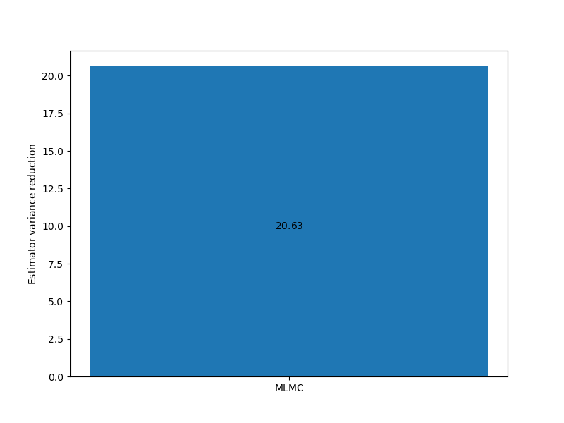
The following compares the estimator variance reduction ratio of MLMC relative to MLMC for a fixed target cost

axs = [plt.subplots(1, 1, figsize=(8, 6))[1]]
# get estimators for target cost = 100
mlmc_est_100 = optimized_estimators[1][1:2]
_ = plot_estimator_variance_reductions(
    mlmc_est_100, est_labels[1:2], axs[0])

The following compares the estimator variance of MC with MLMC for a set of target costs and plot the number of samples allocated to each model by MLMC

# get MLMC estimators for all target costs
mlmc_ests = optimized_estimators[1]
axs[0].set_xlim(target_costs.min(), target_costs.max())
fig, axs = plt.subplots(1, 2, figsize=(2*8, 6))
plot_estimator_sample_allocation_comparison(
    mlmc_ests, model_labels, axs[0])
_ = plot_estimator_variances(
    optimized_estimators, est_labels, axs[1],
    relative_id=0, cost_normalization=1)

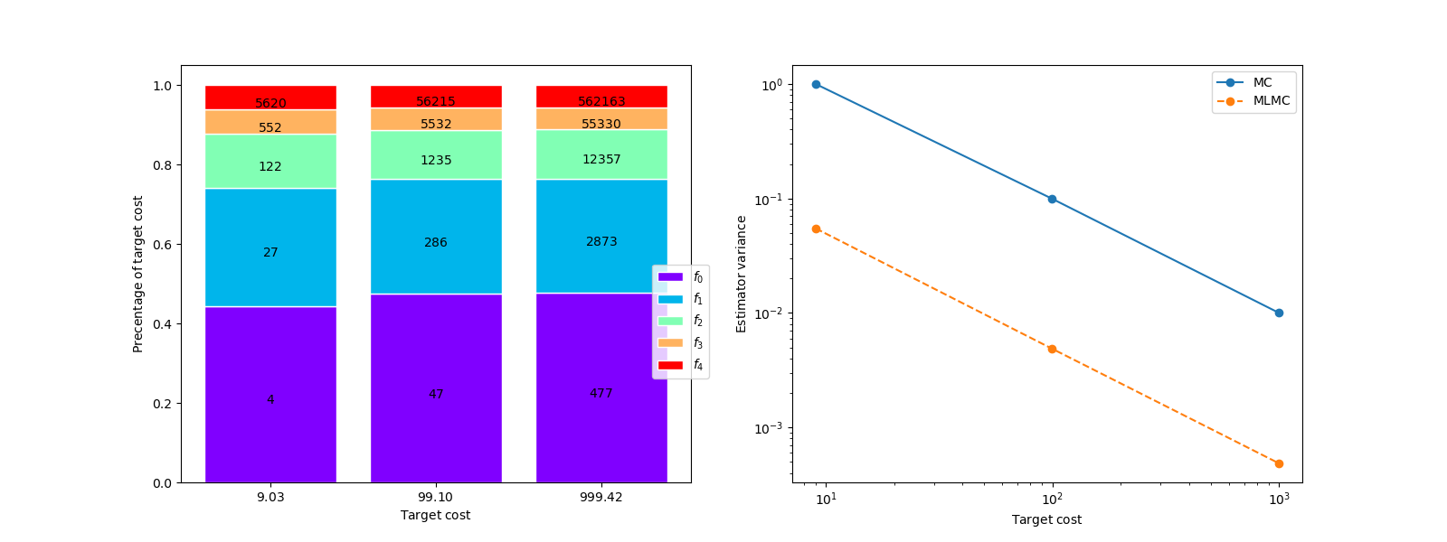
The left plot shows that the variance of the MLMC estimator is over and order of magnitude smaller than the variance of the single fidelity MC estimator for a fixed cost. The impact of using the approximate covariance is more significant for small samples sizes.

The right plot depicts the percentage of the computational cost due to evaluating each model. The numbers in the bars represent the number of samples allocated to each model. Relative to the low fidelity models only a small number of samples are allocated to the high-fidelity model, however evaluating these samples represents approximately 50% of the total cost.

Multi-index Monte Carlo

Multi-Level Monte Carlo utilizes a sequence of models controlled by a single hyper-parameter, specifying the level of discretization for example, in a manner that balances computational cost with increasing accuracy. In many applications, however, multiple hyper-parameters may control the model discretization, such as the mesh and time step sizes. In these situations, it may not be clear how to construct a one-dimensional hierarchy represented by a scalar hyper-parameter. To overcome this limitation, a generalization of multi-level Monte Carlo, referred to as multi-index stochastic collocation (MIMC), was developed to deal with multivariate hierarchies with multiple refinement hyper-parameters [HNTNM2016]. PyApprox does not implement MIMC but a surrogate based version called Multi-index stochastic collocation (MISC) is presented in this tutorial Multi-level and Multi-index Collocation.

The Relationship between MLMC and ACV

MLMC estimators can be thought of a specific case of an ACV estimator. When using two models this can be seen by

\[\begin{split}Q_{0}^\mathrm{ML}(\rvset_0,\rvset_1)&=Y_{0}(\rvset_0)+Y_{1}(\rvset_1)\\ &=Q_{0}(\rvset_0)-Q_{1}(\rvset_0)+Q_{1}(\rvset_1)\\ &=Q_{0}(\rvset_0)-(Q_{1}(\rvset_0)-Q_{1}(\rvset_1))\end{split}\]

which has the same form as the two model ACV estimator presented in Two model Approximate Control Variate Monte Carlo where the control variate weight has been set to \(-1\).

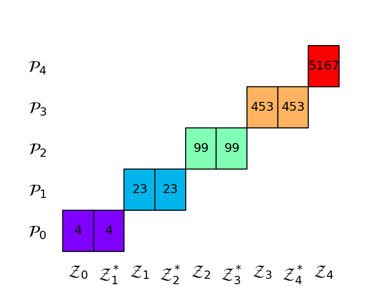
For three models the allocation matrix of MLMC is

\[\begin{split}\mat{A}=\begin{bmatrix} 0 & 1 & 1 & 0 & 0 & 0 & 0 & 0\\ 0 & 0 & 0 & 1 & 1 & 0 & 0 & 0\\ 0 & 0 & 0 & 0 & 0 & 1 & 1 & 0\\ 0 & 0 & 0 & 0 & 0 & 0 & 0 & 1 \end{bmatrix}\end{split}\]

The following code plots the allocation matrix of one of the 5-model estimator we have already optimized. The numbers inside the boxes represent the sizes \(p_m\) of the independent partitions (different colors).

import matplotlib as mpl
params = {'xtick.labelsize': 24,
          'ytick.labelsize': 24,
          'font.size': 18}
mpl.rcParams.update(params)
ax = plt.subplots(1, 1, figsize=(8, 6))[1]
_ = mlmc_ests[0].plot_allocation(ax, True)

MLMC was designed when it is possible to always able to create new models with smaller bias than those already being used. Such a situation may occur, when refining the mesh of a finite element discretization. However, ACV methods were designed where there is one trusted high-fidelity model and unbiased statistics of that model are required. In the setting targeted by MLMC, the properties of MLMC can be used to bound the work needed to achieve a certain MSE if theoretical estimates of bias convergence rates are available. Such results are not possible with ACV.

The following code builds an MLMC estimator with the optimal control variate weights and compares them to traditional MLMC when estimating a single mean.

estimators = [
    get_estimator("mc", stat, costs),
    get_estimator("mlmc", stat, costs),
    get_estimator("grd", stat, costs,
                  recursion_index=range(len(costs)-1))]
est_labels = mathrm_labels(["MC", "MLMC", "MLMC-OPT"])
optimized_estimators = compare_estimator_variances(
    target_costs, estimators)

axs = [plt.subplots(1, 1, figsize=(8, 6))[1]]

# get estimators for target cost = 100
mlmc_est_100 = [optimized_estimators[1][1], optimized_estimators[2][1]]
_ = plot_estimator_variance_reductions(
    mlmc_est_100, est_labels[1:3], axs[0])

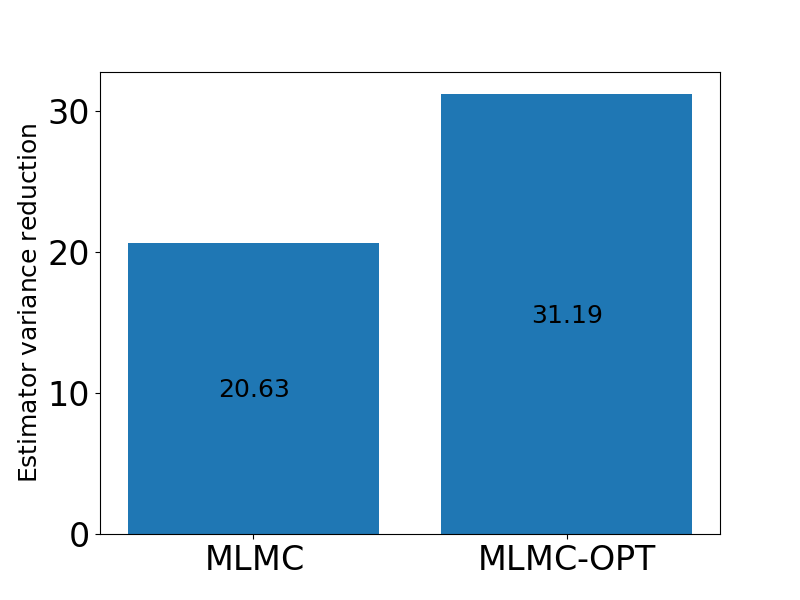
For this problem there is a substantial difference between the two types of MLMC estimators.

Remark

MLMC was originally developed to estimate the mean of a function, but adaptations MMLC have since ben developed to estimate other statistics, e.g. [MD2019]. PyApprox, however, does not implement these specific methods, because it implements a more flexible way to compute multiple statistics which we will describe in later tutorials.

Video

Click on the image below to view a video tutorial on multi-level Monte Carlo quadrature

References

[CGSTCVS2011]

K.A. Cliffe, M.B. Giles, R. Scheichl, A.L. Teckentrup, Multilevel Monte Carlo methods and applications to elliptic PDEs with random coefficients, Comput. Vis. Sci., 14, 3-15, 2011.

[GOR2008]

M.B. Giles, Multilevel Monte Carlo path simulation, Oper. Res., 56(3), 607-617, 2008.

[GAN2015]

M. Giles, Multilevel Monte Carlo methods, Acta Numerica, 24, 259-328, 2015.

[HNTNM2016]

A. Haji-Ali, F. Nobile and R. Tempone. Multi-index Monte Carlo: when sparsity meets sampling. Numerische Mathematik, 132(4), 767-806, 2016.

[MD2019]

P. Mycek, M. De Lozzo. Multilevel Monte Carlo Covariance Estimation for the Computation of Sobol’ Indices. 2019.